

Unit 6 The Phillips curve
The Phillips curve shows how changes in demand can temporarily affect inflation and output as prices adjust over time. In the experiment, participants act as price setters, choosing prices based on demand and their expectations of others, which demonstrates how these individual decisions shape wider economic outcomes.
CORE projects
Concepts in the experiment are related to material in:
6.1 Introduction
The Phillips curve captures the positive relationship between inflation and unemployment in an economy. A central insight is that prices and wages do not adjust instantaneously to shocks. Instead, expectations are often shaped by past experiences, causing inflation to respond only gradually to shocks and creating temporarily higher output and thus lower unemployment.
The game illustrates this mechanism at the micro level. Participants set prices simultaneously while obtaining intermediate inputs from others. They thus engage in forming expectations about the prices chosen by others. Their decisions therefore depend not only on demand but also on their expectations of the behaviour of other participants. When demand increases, prices typically adjust only partially because participants rely on past observations. This creates temporary deviations from equilibrium that are reflected in both inflation and higher output.
By linking individual price-setting decisions to aggregate outcomes, the game provides an intuitive foundation for the Phillips curve and highlights the role of expectations and inflation inertia in macroeconomic adjustment.
How to cite this unit
Giamattei, Marcus, and Johann Graf Lambsdorff (2026). ‘The Phillips curve’. Experiment 6 in The CORE Team, Experiencing Economics. Available at https://www.core-econ.org/experiments/06-the-phillips-curve.html [Accessed on (date)].
Key concepts
This experiment will help students understand the following key concepts:
- Phillips curve
- Inflation inertia
- Price-setting
- Adaptive expectations
- Demand shocks
6.2 Requirements
Timing
The game consists of ten rounds with one decision per player each round. It can be run in 30 minutes (including some introductory explanation).
Remember to allow time for a stimulating discussion.
6.3 Description of the experiment
In this experiment, each participant represents a producer in an economy. In each of the ten rounds, participants choose a price, \(p\), for their product simultaneously with all other participants.
6.4 Step-by-step guide
Detailed instructions
Go to the ‘Quick summary’ section if you have previously run the experiment and just need a brief reminder of the instructions.
6.5 Student instructions
These are also available in the students’ version.
A PDF of the student instructions and homework questions is also available.
Each participant represents a producer in an economy. In each of the ten rounds, your only task is to determine a price \(p\) for your product. At the same time, the other participants determine the price of their product. By choosing \(p\), you determine the level of demand according to the function:
\[y = \omega - p\]The lower the price you choose, the greater the demand, \(y\). It increases with the exogenous influence \(\omega\), which indicates the maximum possible demand at a price of \(p = 0\). Each participant automatically produces as much as is demanded.
Each producer purchases intermediate goods from other producers at prices determined by those producers. The capital letter \(P\) denotes the average of the prices of all producers. This average determines your unit costs. These are \(P - 10\) and the total cost of the entire production therefore amounts to \(y \times (P - 10)\). Profit is calculated as sales minus costs, that is
\[y \times p - y \times (P - 10)\]The average price, \(P\) is necessarily unknown at the beginning of a round. This means that when you set the price of your product, you do not yet know the cost of your production, as this depends on the prices of all other producers.
The game is played over ten rounds. In the first five rounds, \(\omega = 30\). In the second five rounds, \(\omega = 50\).
Individual participants achieve high profits when production and profit per unit do not differ greatly.
This is shown in Figure A, which depicts the demand curve for \(\omega = 30\). It also shows the costs per unit \(P - 10\). As the demand curve reflects the price, the difference between the two curves is the profit per unit. Total profit is reached by multiplying with the quantity produced. Therefore, total profit is represented by the rectangle in Figure A. Maximizing this rectangle implies making it quadratic.
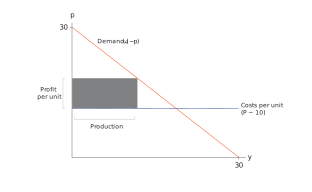
Figure A Visualization.
Your screen in the experiment will look like Figure B. You are given the demand and the cost function and you are asked to enter your price, \(p\).
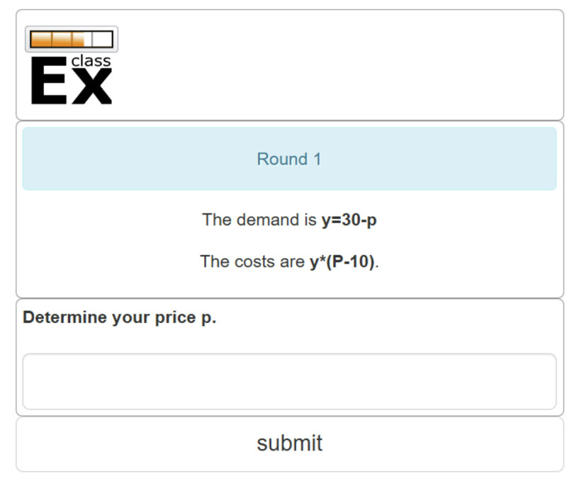
Figure B Price input screen.
After all participants have set their price, you will receive feedback on the average price set by the participants, and your payoff you gained in that round (your ‘income’). This is shown in Figure C. It also shows the solution in a graphical way.
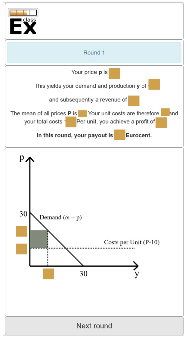
Figure C The classEx feedback screen.
It is very important that you abide by the following rule: All your decisions must be kept private. You must not communicate with other students nor make public announcements, no matter how tempting it might become.
Warm-up questions
You can use the following questions to test your understanding of the rules.
- What is your decision in each round?
- A. How much to produce
- B. Which price to set
- C. What the average price will be
- D. How much to pay other producers
- If you choose a lower price, what happens to demand for your product?
- A. Demand increases
- B. Demand decreases
- C. Demand stays the same
- D. Demand becomes zero
- What does \(P\) represent in the experiment?
- A. Your own price
- B. The highest price chosen by any producer
- C. The average price chosen by all producers
- D. Your profit
- Why do you not know your exact production costs when you choose your price?
- A. Because demand is random
- B. Because costs depend on the average price chosen by all participants
- C. Because \(\omega\) is unknown
- D. Because production is chosen after the round
- Unit costs are given by: \(P - 10\). If the average price is \(P = 18\), what are your unit costs?
- Profit is calculated as: \(y \times p - y \times (P - 10)\). If your demand is \(y = 20\), your price is \(p = 15\), and the average price is \(P = 18\), what is your profit?
- B
- A
- C
- B
- \(18 - 10 = 8\)
- \(\text{Profit} = 20 \times 15 - 20 \times 8 = 300 - 160 = 140\)
6.6 Predictions
Predicted results
As shown above, with rational expectations, all participants will come to the same result, with \(p = \omega - 10\) and \(y = 10\). This means that production is constant in equilibrium, that is, independent of the exogenous influence \(\omega\), as shown in Figure 6.6 by a vertical, dashed line. This line is sometimes called a long-term Phillips curve, where quantities are fixed and changes only take place with prices.
6.7 Discussion
A good discussion following the experiment is important. Ask your students the following questions to frame the discussion.
Interpreting the graphs
- How does the line representing the prices chosen by the participants behave?
- What influence did the demand shock have on this line?
6.8 Homework questions
These questions can be set for students to work on outside the classroom or can be completed and discussed in the classroom. They may help students reflect on their experience and understand their and others’ behaviour in the experiment.
Data from your experiment can be downloaded as an Excel file from the ‘data’ menu in the instructor’s screen in classEx. You can use this data to create your own questions. A description of the data variables can be found in the ‘Downloading the data from your experiment’ section.
The following text is also available in the students’ version.
- Assume that the demand, \(y\), for products from a representative producer in an economy is given by \(y = \omega − 2p\) and that production corresponds to demand. The costs amount to \(y \times (P − 40)\), where \(P\) is the price of the basket of all products in the economy.
- Determine the optimal price, \(p\), as a function of the price of the basket of goods, \(P\).
- Determine the optimal price in the event that all other producers also choose this price.
- Assume that \(\omega = 480\) in the first five rounds and \(\omega = 680\) in the remaining five rounds. Calculate the optimal price and quantity in each round.
- Figure D shows the prices and quantities chosen by participants in a lecture hall in 2022 for a similar task. In Round 6, \(\omega\) increased. Why did production increase in Round 6? How can the chosen prices be explained by sticky information or limited rationality?
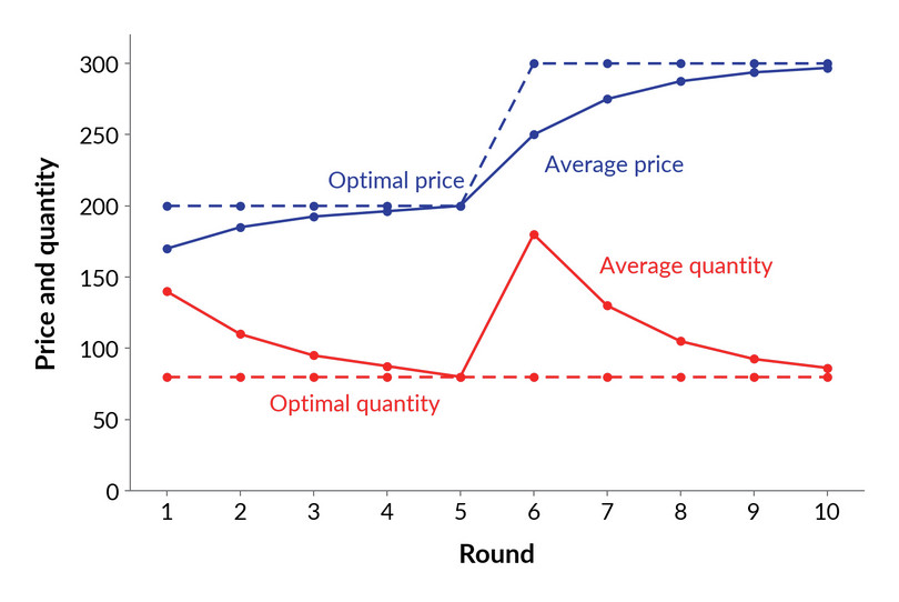
Figure D Results from a run of the classEx game.
