Experiment 7 Network economies of scale: The Holophone
7.1 Introduction
CORE projects
Concepts in the experiment are related to the material in:
Have you ever wondered about the significance of being the first person with email access, only to find an empty inbox? Why did some social networks succeed and become giants (like Facebook), while others offering similar services failed to take off (like Google+ or MySpace)? Many communication devices like the telegraph, the telephone, or email were a marginal product for a fairly long time until they enjoyed a period of explosive growth that made them ubiquitous. Their growth followed a hockey stick path. More recently, social networks (like Facebook, Instagram, LinkedIn, Snapchat, or Pinterest) or delivery platforms (like Uber Eats, Instacart, or Globo) show a similar evolution. All these goods and services have a common characteristic: they exhibit network economies of scale, that is, the value they provide to customers increases with the number of users or members.
This is a simple, and fast to run, experiment in which students must decide whether or not to buy a new product that is competitively offered at a fixed price, and whose value for consumers increases with the number of purchases. Students have an initial value that reflects how much they like the good per se, but they cannot know their final buyer values until the market closes and the total number of buyers is determined. During each round, the number of units bought is publicly announced in real time, so students may decide to wait until there are enough users to make buying a profitable decision for them. However, if everybody waits for others to buy, the round ends with no sale or too few sales for buyers to make a profit.
The experiment is played for different prices, and all rounds (apart from the first) present two equilibria: one where no units are sold, and another where high sales are achieved. Which one occurs depends on the decisions of participating students and, in particular, on whether a critical mass is reached. The experiment’s multiple equilibria offer a simple setting to discuss equilibrium dynamics and stability. (See also the second homework question in Section 7.8.) The critical mass observed in this experiment parallels the tipping point in the environmental dynamics curve discussed in Section 20.8 of The Economy 1.0.
A graph at the end of the experiment shows the path of purchases, which usually reproduces a hockey stick growth path for the round where a critical mass has been attained.
This experiment can be easily combined in the same session with the experiment Competing Standards. Both experiments share a similar mechanism and students can use what they learned by reading the instructions of this experiment to participate in the other.
This experiment is an adaptation of ‘Network Externalities’ from Experiments with Economic Principles: Microeconomics by Ted Bergstrom and John Miller.
Citation: Llavador, Humberto, Marcus Giamattei, Ted Bergstrom, and John H. Miller. 2023. ‘Network economies of scale: The Holophone’. Experiment 7 in The CORE Team, Experiencing Economics. Available at https://www.core-econ.org/experiencing-economics.
Key concepts
This experiment will help students understand the following key concepts:
- network economies of scale
- network externalities
- critical mass
- stable equilibrium
- unstable equilibrium.
7.2 Requirements
Timing
This is a quick experiment to run, once students have understood the rules of the game. You can conduct all rounds in 5 to 10 minutes, depending on the number of participating students and how fast they reach critical mass. Understanding the instructions requires some time, though, but you can speed up the process by providing students with access to the instructions and the warm-up questions beforehand. The experiment can be run in the classroom or online. When run online, critical mass tends to be reached faster and the expansion of the network is not as visual as in the classroom.
7.3 Description of the experiment
In this experiment, students must decide (in each round) whether to buy a new type of phone that communicates through holographic images. We call it a Holophone. Their objective is to maximize their payoff, that is, the difference between their buyer value and the price paid for the Holophone, in each round. Rounds are treated as independent decisions and payoffs do not accumulate. The price is set and announced at the beginning of each round by the instructor, who is the only supplier of Holophones. Students are assigned an initial value (from 1 to 6), which represents how much they like the Holophone as a gadget. However, buyer values will also depend on usability, and hence on the number of other students who have bought a Holophone by the end of the round, since Holophone owners can only communicate with other Holophone owners.
7.4 Step-by-step guide
Detailed instructions
Go to the ‘Quick summary’ section if you have previously run the experiment and just need a brief reminder of the instructions.
7.5 Student instructions
These are also available in the students’ version.
A PDF of the student instructions and homework questions is also available.
Introduction
Having your own phone is not of much use if your friends do not have phones. And what use is it to have an email account if the people you want to send messages to do not have email accounts too? The technology for the fax, a device to send images of documents over a telephone line, was first patented by Alexander Bain in 1843, but fax machines were still rare as late as 1980. Suddenly, they became so popular that by the mid-1980s almost every office had at least one fax machine. A defining characteristic of this type of good is that it becomes more valuable to everyone as more people purchase it.
This experiment explores the workings of a market for such a good. It introduces the Holophone:1 a smartphone that communicates with holographic images. It is a more advanced way of communicating, but you can communicate with someone only if both of you have Holophones. Will Holophones make smartphones a thing of the past or will they fade away and make buying them a waste of money?
Instructions
The network externality factor represents the benefits of one user on another, occurring because the two are connected in a network.
In this experiment, you will take part in a market of Holophones. Your task is to make a decision whether to purchase a Holophone at an announced price or not, with the aim of maximizing your payoff. The payoff is determined by the difference between the price paid and your buyer value. Your buyer value will be determined by two factors: your initial value and the usability of the Holophone, measured by the network externality factor (NEF), which is determined by the number of other participants who also have a Holophone.
At the beginning of the experiment, you are informed of your initial value—that is, how much you value a Holophone even if nobody else has one. (About one-sixth of participants have each of the possible initial values ranging from 1 to 6.) However, you will not know your buyer value until the end of the round, since it is contingent on both your initial value and the total number of Holophones sold, according to the following formula:
\[\text{buyer value = initial value} \times \text{network externality factor (NEF)}\]The NEF is determined by the total number of participants who buy a Holophone according to a conversion table that will be displayed at the beginning of the session. The NEF table and your initial value are maintained for all rounds.
In each round of this experiment, the instructor, who is the only seller, will announce the price of a Holophone. The price is the same for the entire round. You will see the number of units sold on your instructor’s screen, as buying orders start coming. If you want to buy a unit, you need to send the order through your device (Figure A). Your instructor may also ask you to stand up or move to a designated area in the room to provide a more visual picture of the number of phones sold. Observe that you can only buy one unit or none, and that it is not possible to change the decision once you have sent it.
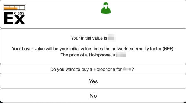
Figure A Student’s screen showing the information on the initial value and price (hidden), and the buttons to buy or not to buy.
Once the round is closed, the NEF is calculated and you will receive feedback with your buyer value and your profits (or losses), that is, your buyer value minus the price you paid. If you decide not to buy, you will receive a profit of zero. Zero profits are better than obtaining a loss by paying a price higher than your buyer value.
It is very important that you abide by the rules described by your instructor. In particular, you must not make public announcements, no matter how tempting it might become.
Warm-up questions
You can use the following questions to test your understanding of the rules.
Suppose that the network externality factors (NEF) are as given in Figure B.
| If the number of units sold is between | NEF is |
|---|---|
| 0 and 8 | 1 |
| 9 and 16 | 2 |
| 17 and 24 | 3 |
| 25 and 32 | 4 |
| 33 and 40 | 5 |
| 41 or more | 6 |
Figure B Example of network externality factors (NEF) table for the training questions.
- Suppose 11 students bought a Holophone.
- What is the NEF?
- Suppose that Holophones sell for €20 and your initial value is 6. If you were one of the buyers, what would be your profit or loss?
- Suppose that Holophones sell for €12, that 36 students have already bought a Holophone, and that you will be the last student to buy.
- If your initial value is 3, what would be your profit (loss) from buying a Holophone?
- If your initial value is 2, what would be your profit (loss)?
- Suppose that Holophones sell for €8. Your initial value is 3, and 16 students have already bought a Holophone. Should you buy?
- Your initial value is 3, and you bought a Holophone for €5. What is the minimum number of units that other students must buy for you to make a strictly positive profit?
-
- NEF = 2
- Your buyer value is \(6\times 2 = €12\). Since you paid €20, you lose €8.
-
- With 37 users, including yourself, NEF = 5 and your buyer value is \(3\times 5 = €15\). Since you pay €12, your profits are €3.
- Now, your buyer value is \(2\times 5 = €10\), and you lose €2.
- If you buy one unit, there will be 17 users, including yourself. NEF = 3, your buyer value will be \(3\times 3 = €9\), and your profits \(=9-8=€1\).
- To make a strictly positive profit, you need a buyer value of €6 or higher. Since your initial value is 3, the NEF must be at least 2. That is, a minimum of eight other students must buy a unit.
7.6 Predictions
Predicted results
At the default price of €20, Rounds 1 and 2 should end with no units sold. It is common to have a few bold pioneers (not always students with the highest initial values) buying a unit. But those who bought lost money and would like to return the Holophone if they could. (With a NEF of 1, the highest buyer value would be only €6, which is much less than the cost of a unit.)
7.7 Discussion
A good discussion during and after the experiment is important. Ask your students the following questions to frame the discussion.
Comments in the ‘Predictions’ and ‘What might go differently?’ sections, and in The Economy 1.0 (Section 21.4) provide useful further information.
Interpreting the graph
These questions refer to the time graph displayed by classEx at the end of the experiment.
7.8 Homework questions
These questions can be set for students to work on outside the classroom or can be completed and discussed in the classroom. They may help students reflect on their experience and understand their and others’ behaviour in the experiment.
For the numerical questions, you will need to provide your students with the following information: the network externality factors table (from the table in Figure 7.8); the distribution of initial values (from table in Figure 7.7); and the price, number of units sold, and network externality factor for each round (from a screenshot of the instructor’s screen at the end of the experiment or from the data file downloadable from classEx).
Data from your experiment can be downloaded as an Excel file from the ‘Data’ menu in the instructor’s screen in classEx. You can also use this data to create your own questions. A description of the data variables can be found in the ‘Downloading the data from your experiment’ section.
The following text is also available in the students’ version.
Your instructor shared with you the following information regarding the experiment: the network externality factors table; the distribution of initial values; and the price, the number of units sold, and the network externality factor for each round.
A. Finding equilibria with a no-regrets demand curve
Drawing the no-regrets demand curve
When we draw a demand curve for a good with network economies of scale, it is convenient to do so by finding the price(s) at which each quantity will be demanded. This is so because when there are network economies of scale, each person’s buyer values depend on the total number of units sold. For each quantity \(q\), define \(P(q)\) to be the buyer value of ‘the last buyer’ when exactly \(q\) units are sold.2
- Observe that, because all buyers share the same NEF, the ‘last buyer’ is the buyer with the lowest initial value: participants with higher initial values should buy first. Because there are six different initial values, there are six ranges of quantities such that \(P(q)\) is constant over each range. Complete the table in Figure C for these ranges for the different values of \(P(q)\).
| Quantity range | Network externality factor NEF | Lowest initial value (decreasing sorted) IV(q) | P(q) in this range NEF × IV(q) |
|---|---|---|---|
| 1 to _ | 1 | 6 | €6 |
| _ to _ | 2 | 5 | €10 |
| _ to _ | 3 | 4 | €12 |
| _ to _ | 4 | 3 | €12 |
| _ to _ | 5 | 2 | €10 |
| _ to _ | 6 | 1 | €6 |
Figure C Table for \(P(q)\).
- Use the first and last columns in Figure C to draw a graph of the no-regrets demand curve \(P(q)\). Add a vertical line segment corresponding to zero sales at each price above €6, and draw vertical line segments to fill in the jumps between the horizontal line segments in your graph of \(P(q)\). Your graph should look like the one in Figure D.

Figure D Example of no-regrets demand curve.
Finding the equilibria
- On your graph, draw a horizontal supply curve at a price of €20. What is the equilibrium quantity at this price?
- In Round 2, the price was €20. How many units were sold in this round? How many of the buyers made positive profits? How many of the buyers took losses? If there had been a third round where the price was still €20, how many Holophones do you think would have been sold?
- On your graph, draw (perhaps using a different colour) a horizontal supply curve at a price of €11. What are the equilibrium quantities with this new supply curve?
- In Round 3, the price was €11. How many units were sold? Is the quantity outcome of the round closer to ‘low level’ or to the ‘high level’ of the equilibria you found for a price of €11?
- If your group ran Round 4, repeat questions 5 and 6 for a price of €9 (the price of a unit in Round 4).
Stability of equilibria
- Suppose that the price is €11 and the market is stuck to the low-level equilibrium where nobody buys a Holophone. The market reopens and only one or two students buy a unit. Will they get positive profits? Would they return the unit and get their money back if they could? Observe that for small deviations, the dynamics pull the situation back to the low-level equilibrium.
- The price is still €11, but suppose now that the market has attained the high-level equilibrium. A new opportunity arises for buyers to change their mind. Those who did not buy a Holophone can buy one unit, and those who bought one unit may return it and get their money back. Check whether (a) if anyone returned a Holophone, they would buy it back; and (b) if there were one more sale, the buyer would return it. Observe that, for small deviations, the dynamics pull the situation back to the high-level equilibrium.
- Finally, suppose that the price is €9 and that the market is stuck at the low-level equilibrium where nobody buys a Holophone. The government is interested in the expansion of the use of these new devices and decides to subsidize \(k\) units which are offered at a reduced price of €5 each, where \(k\) is the number of students with an initial value of 6. What do you think would happen to the total number of units sold? (If your group ran Round 5, compare your answer to the outcome of that round.)
B. An example with a large number of users
In this example, we extend the analysis to a very large number of users. Consider the pool of smartphone owners. A new video and file-sharing network is launched. The value to each owner of joining this new network depends on their personal interest to join in (their initial value) and the fraction of users (that is, those smartphone owners who have already joined). We identify each owner by a number in the interval from 0 to 1, with 0 and 1 representing the most- and the least-interested owner, respectively. In particular, the initial value of owner \(q\) is \((1-q)\), and if a share \(k\in [0,1]\) of owners joins the network, the buyer value of user \(q\) is \((1-q)\times k\). For example, if the share of users is 50% (\(k=0.5\)), the buyer value of owner \(q=0.3\) (who has the highest 30% initial value) is \(0.7 \times 0.5=0.35\), that is, they would be willing to pay up to 0.35 euros to join the network.
- Suppose that the cost of joining the network is €0.21. Hence, everybody whose buyer value \(\geq 0.21\) would like to join. If 50% of owners have already joined, compute the share of owners who would like to join the network by solving the equation \((1-q)\times 0.5= 0.21\). We will call them the expected users.
- Using a graphic calculator (like Geogebra), draw the share of expected users as a function of the number of actual users (\(k\)). Recall that the price is €0.21 and notice that the share of expected users cannot be less than 0.
- On the same graph, draw the 45° line through the origin and find the intersections of both functions. You should obtain a graph similar to Figure E. Each intersection represents an equilibrium, because the expected share of users coincides with the actual share of users. (You could also compute the equilibria analytically.)

Figure E Expected users as a function of current users. Points A, B, and C represent different equilibria.
Now, let’s study the dynamics off-equilibrium.
- Suppose that the actual share of users is to the left of point B. Find the expected number of users, who will become the new share of users. Continuing this argument, show that the dynamics will lead to point A with no users.
- Repeat the previous argument for a share of users between points B and C, and for a share of users to the right of point C.
- Using questions 4 and 5, argue that A and C represent stable equilibria, while B is an unstable equilibrium.
- If you want to practice more, repeat the whole analysis for other prices, for example \(p=0.09\), \(p=0.25\), or \(p=0.3\). You will discover that for prices higher than €0.25, the only equilibrium is no users.
7.9 Further reading
Also available in the students’ version.
- Section 7.3 in The Economy 2.0: Microeconomics (Section 7.2 in The Economy 1.0) and Section 21.4 in The Economy 1.0, discuss the concept of network economies of scale. Section 20.8 in The Economy 1.0 presents an analysis of the stability of equilibria applied to an environmental context, where tipping points play the role of the critical mass in this experiment. Section 1.2 in The Economy 2.0: Microeconomics (Section 1.3 in The Economy 1.0) introduces the hockey stick concept to describe a time graph.
- The discussion of Experiment 9 ‘Network Externalities’ in Theodore Bergstrom and John Miller. 2000. Experiments with Economic Principles: Microeconomics (2nd ed.). McGraw-Hill Education, pp. 255–266 still offers an excellent theoretical analysis of network economies of scale particularly tailored to this experiment.
- Ernie G.S. Teo. 2015. ‘Emergence, Growth, and Sustainability of Bitcoin: The Network Economics Perspective’. (chapter 9.1 in The Handbook of Digital Currency, edited by David Lee Kuo Chuen, Academic Press) discusses network effects and how they affect a cryptocurrency’s emergence and growth.
- J. C. Coopersmith. 2014. ‘STARS: Fax Machines [Scanning our Past]’ (in Proceedings of the IEEE 102 (11): pp. 1858–1865.doi: 10.1109/JPROC.2014.2360032) shows how the fax machine turned from being a niche product for more than a hundred years to become, within the space of ten years, an indispensable machine in almost every office.
