
Unit 3 Work, scarcity, and choice
How individuals do the best they can, and how they resolve the trade-off between working in the labour market and other activities
- opportunity cost
- When taking an action implies forgoing the next best alternative action, this is the net benefit of the foregone alternative.
- Decision making under scarcity is a common problem because we usually have limited means available to meet our objectives.
- Economists model these situations, first by defining all of the feasible actions people can take and then evaluating which of these actions is best, given the objectives.
- Opportunity costs describe the unavoidable trade-offs in the presence of limits: satisfying one objective more implies satisfying other objectives less.
- A model of decision making can be applied to the question of how much time to spend working, when facing a trade-off between more income from working and time to do other activities.
- This model also helps to explain differences in the hours that people work in different countries, and the changes in our hours of work throughout history.
Imagine that you are working in New Delhi, in a job that is paying you Rs. 40 an hour for a 40-hour working week, which gives you earnings of Rs. 1,600 per week. There are 168 hours in a week, so after 40 hours of work, you are left with 128 hours of free time for all your non-work activities, including leisure and sleep.
Suppose, by some happy stroke of luck, you are offered a job at a much higher wage—six times higher. Your new hourly wage is Rs. 240. Not only that, your prospective employer lets you choose how many hours you work each week.
Will you carry on working 40 hours per week? If you do, your weekly pay will be six times higher than before: Rs. 9,600. Or will you decide that you are satisfied with the goods you can buy with your weekly earnings of Rs. 600? You can now earn this by cutting your weekly hours to just 6 hours and 40 minutes (a six-day weekend!), and enjoy about 26% more free time than before. Or would you use this higher hourly wage rate to raise both your weekly earnings and your free time by some intermediate amount?
The idea of suddenly receiving a six-fold increase in your hourly wage and being able to choose your own hours of work might not seem very realistic. But we know from Unit 2 that technological progress since the Industrial Revolution has been accompanied by a dramatic rise in wages. In fact, the average real hourly earnings of American workers did increase more than six-fold during the twentieth century. And while employees ordinarily cannot just tell their employer how many hours they want to work, over long time periods the typical hours that we work do change. In part, this is a response to how much we prefer to work. As individuals, we can choose part-time work, although this may restrict our job options. Political parties also respond to the preferences of voters, so changes in typical working hours have occurred in many countries as a result of legislation that imposes maximum working hours.
So have people used economic progress as a way to consume more goods, enjoy more free time, or both? The answer is both, but in different proportions in different countries. While hourly earnings increased by more than six-fold for twentieth century Americans, their average annual work time fell by a little more than one-third. So people at the end of this century enjoyed a four-fold increase in annual earnings with which they could buy goods and services, but a much smaller increase of slightly less than one-fifth in their free time. (The percentage increase in free time would be higher if you did not count time spent asleep as free time, but it is still small relative to the increase in earnings.) How does this compare with the choice you made when our hypothetical employer offered you a six-fold increase in your wage?
How has the number of hours that people have spent working changed over the last century and a half? Figure 3.1 shows trends in income and working hours since 1870 in three countries.
As in Unit 1, income is measured as per-capita GDP in US dollars. This is not the same as average earnings, but gives us a useful indication of average income for the purposes of comparison across countries and through time. In the late nineteenth and early twentieth century, average income approximately trebled, and hours of work fell substantially. During the rest of the twentieth century, income per head rose four-fold.
Hours of work continued to fall in the Netherlands and France (albeit more slowly) but levelled off in the US, where there has been little change since 1960.
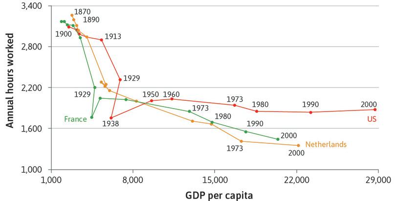
Figure 3.1 Annual hours of work and income (1870–2000).
Maddison Project. 2013. 2013 edition. Michael Huberman and Chris Minns. 2007. ‘The times they are not changin’: Days and hours of work in Old and New Worlds, 1870–2000’. Explorations in Economic History 44 (4): pp. 538–567. GDP is measured at PPP in 1990 international Geary-Khamis dollars.
Over this period, incomes have risen, as we can see, quite extensively. Did societies use this progress to consume more goods, enjoy more free time, or both? The answer is both, but in different proportions in different countries. While many countries have experienced similar trends, there are still some differences in outcomes. Figure 3.2 illustrates the wide disparities in income and time off from paid work between countries in 2013. Here we have calculated free time by subtracting average annual working hours from the number of hours in a year. You can see that the higher-income countries seem to have lower working hours and more free time, but there are also some striking differences between them. For example, the Netherlands and the US have similar levels of income, but Dutch workers have much more time outside paid work. And the US and Turkey have similar amounts of free time but a large difference in income.
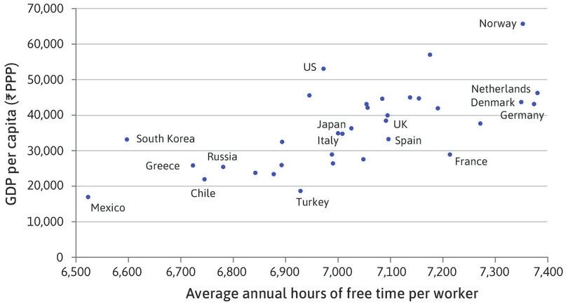
Figure 3.2 Annual hours of free time per worker and income (2013).
OECD. Average annual hours actually worked per worker. OECD. Level of GDP per capita and productivity. Accessed June 2016. Data for South Korea refers to 2012.
In many countries there has been a huge increase in living standards since 1870. But in some places people have carried on working just as hard as before but consumed more, while in other countries people now have more free time. How does one account for these differences? The full answer is complex and depends on many things. Demographic differences mean that in some countries more people are of working age. Political and cultural arrangements and agreements between workers and owners mean that in some countries, time off from paid work is more easily available.
- scarcity
- A good that is valued, and for which there is an opportunity cost of acquiring more.
Why has this happened? We will provide some answers to this question by studying a basic problem of economics—scarcity—and how we make choices when we cannot have all of everything that we want, such as goods and free time. But before we do this we begin by describing how work itself is organized and how it differs across societies.
Question 3.1 Choose the correct answer(s)
Currently you work for 40 hours per week at the wage rate of Rs. 20 an hour. Your free hours are defined as the number of hours not spent in work per week, which in this case is 24 hours × 7 days − 40 hours = 128 hours per week. Suppose now that your wage rate has increased by 25%. If you are happy to keep your total weekly income constant, then:
- The new wage rate is Rs. 20 × 1.25 = Rs. 25 per hour. Your original weekly income is Rs. 20 × 40 hours = Rs. 800. Therefore, your new total number of working hours is Rs. 800/Rs. 25 per hour = 32 hours. This represents a change of (32 – 40)/40 = −20%.
- The new wage rate is Rs. 20 × 1.25 = Rs. 25 per hour. Your original weekly income is Rs. 20 × 40 hours = Rs. 800. Therefore, your new total number of working hours is Rs. 800/Rs. 25 per hour = 32 hours.
- The new wage rate is Rs. 20 × 1.25 = Rs. 25 per hour. Your original weekly income is Rs. 20 × 40 hours = Rs. 800. Therefore, your new total number of working hours is Rs. 800/Rs. 25 per hour = 32 hours. Then your free time is now 24 hours per day × 7 days per week – 32 = 136 hours per week, an increase of (136 – 128)/128 = 6.25%.
- The new wage rate is Rs. 20 × 1.25 = Rs. 25 per hour. Your original weekly income is Rs. 20 × 40 hours = Rs. 800. Therefore, your new total number of working hours is Rs. 800/Rs. 25 per hour = 32 hours. Then your free time is now 24 × 7 – 32 = 136 hours per week, an increase of (136 – 128)/128 = 6.25%.
Question 3.2 Choose the correct answer(s)
Look again at Figure 3.2, which depicts the annual number of hours worked against GDP per capita in the US, France and the Netherlands, between 1870 and 2000. Which of the following is true?
- The negative relationship between the number of hours worked and GDP per capita does not necessarily imply that one causes the other.
- The lower GDP per capita in the Netherlands may be due to a number of factors, including the possibility that Dutch people may prefer less income but more leisure time for cultural or other reasons.
- The GDP per capita of France increased from roughly to $2,000 to $20,000 (ten-fold) while annual hours worked fell from over 3,000 to under 1,500.
- That would be nice. However past performance does not necessarily mean that the trend will continue in the future.
3.1 Work and its forms
Work takes many forms. It can be paid or unpaid. It might be performed at home or in a workplace, such as a shop, an office, or a factory. It can be done with different social regulations, often within the same country or region. Some people are employed on a regular monthly salary, others earn from day to day as casual workers, others operate their own businesses and are considered self-employed. For most people work is the primary source of income and survival.
- own account work
- Work undertaken for oneself, rather than for an employer.
- piece-rate work
- A type of employment in which the worker is paid a fixed amount for each unit of the product made.
Paid work also takes many forms. The most common form of paid work in high-income countries is wage work. In low-income countries like India, a large category of paid work is own account work or work in a family enterprise. For example, a woman working by herself or with her family, doing embroidery or raising livestock, or a man running a small shop by himself or with his wife. Often such self-employed workers may work for a contractor on piece-rates, but retain some autonomy over their time.
- casual labour
- People who are employed on a temporary, rather than a permanent or regular basis.
The second most common form of paid work in low-income countries is casual labour, performed for a daily wage. Daily wage workers do not have secure employment. They try their luck in the labour market every day. On any given day, some fraction of them will find work while others return home without a day’s wages. Agricultural workers, carpenters, painters, masons, and other construction workers often participate in such markets.
- regular wage
- A fixed and regular compensation for services provided, independent of time taken to provide those services.
The rarest and the most sought-after type of work is regular wage or salaried employment. This is the form of work that we often think of when we use words such as ‘job’ or ‘employment’. But the truth is that such workers are a small minority of the world’s workforce, even if they are the majority of the workforce in high-income countries.
In low-income countries, work also differs a great deal in terms of its productivity, or value generated per unit time. Very tiny scales of operation are common in all sectors of the economy and levels of mechanisation are low. This means that a whole day of hard work may generate much less value than an equivalent time spent in a modern workshop, factory, or office where workers have access to the latest technology. Certainly, productivity differences as we have seen in Unit 2 between countries are large, but they are also large within low-income countries. Such differences in productivity, both within and between countries, accounted for by levels of education, skills, and automation, often lie behind earning inequalities in the developing world.
Whether or not people have been involved in paid work has also depended on another fundamental and perhaps less obvious feature: one’s gender. In many, perhaps most, societies women do not participate in the labour force to the same extent as men. This is not to say that they work any less, but rather that much of their work is unpaid.
Various types of paid and unpaid work may be performed by a person, sometimes even in a day or a week. For example, a woman may perform care work, undertake paid embroidery work and help out on the family farm, all in one day. To take another case, a person may be a casual or daily wage worker a few times a week and on days when such work is not available, may help out in their neighbour’s store, perhaps for remuneration in kind (such as meals for the day).
- caring labour
- Labour which is undertaken out of affection or a sense of responsibility for other people, with no expectation of immediate pecuniary reward.
Work performed at home, like taking care of children, cooking meals, doing the laundry, looking after the sick or the elderly, is called care work. Time spent in this work can be a significant portion of the day, especially for women. This work is vital for the reproduction of human society. But it is unpaid and often undervalued. Recent research shows that the burden of such work is also a serious constraint on women’s ability to work for pay. Even when women experience no cultural norms preventing them from working for pay, domestic responsibilities may prevent them from doing so.
Figure 3.3 and Figure 3.4 give an indication of the difference in paid work for women and men. Figure 3.3 shows the fraction of women and men who were part of the labour force (i.e. were looking for or had paid jobs) from 1900 to 2000 in five high-income countries. Throughout the twentieth century women participated more and more in the labour force, while men’s participation declined. Still, in 2000 in all five countries, women had a lower labour force participation rate than men.
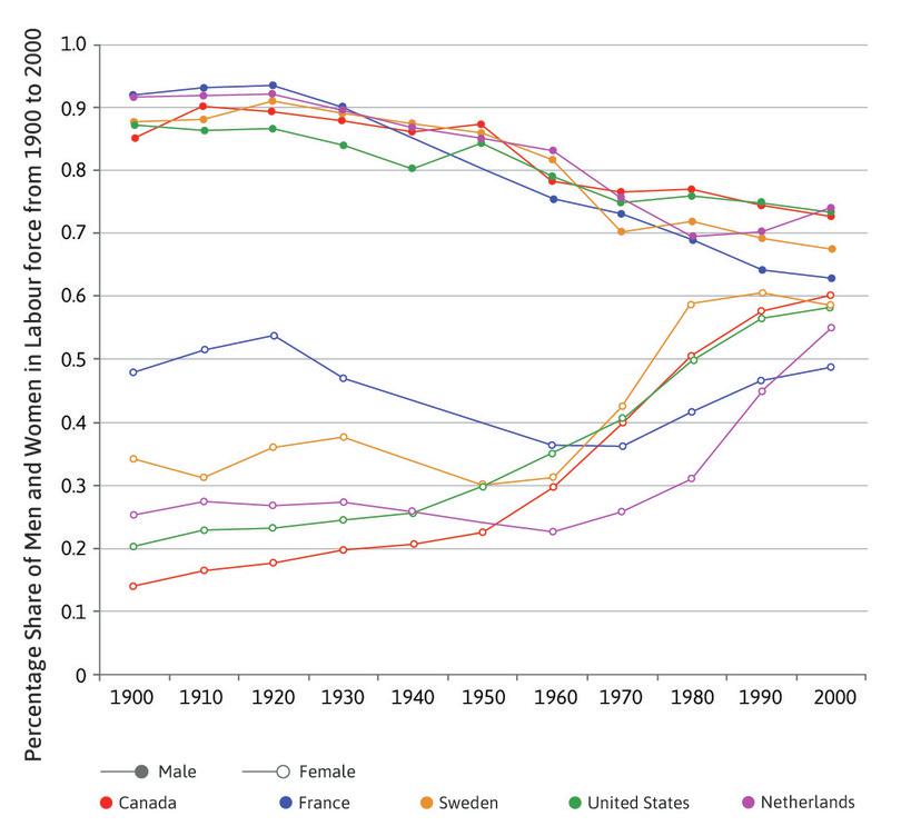
Figure 3.3 Share of men and women in labour force from 1900 to 2000.
Olivetti, Claudia. 2014. ‘The Female Labor Force and Long-Run Development: The American Experience in Comparative Perspective’. In Human Capital in History: The American Record by National Bureau of Economic Research, eds. Leah Platt Boustan, Carola Frydman, and Robert A. Margo. Chicago: University of Chicago Press.
Figure 3.4 shows the results of a ‘time use survey’ done across several countries in 2014. In all cases women spent more time in unpaid work (cooking, cleaning and child care) than men. In India, for example, women spent six times more time than men in such tasks.
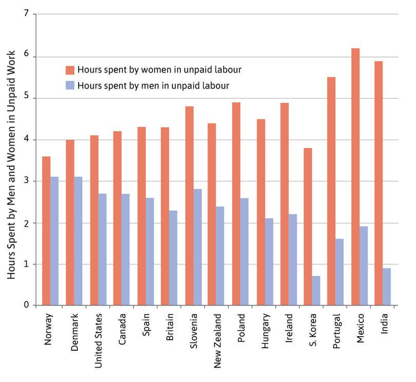
Figure 3.4 Hours spent by men and women in unpaid work.
OECD. Time spent in paid and unpaid work, by sex. Accessed March 2020. The countries are arranged in ascending order by the size of the ratio of women’s to men’s time spent in unpaid labour. Norway has the lowest ratio and India has the highest.
Exercise 3.1 Caring labour
Note that in Figure 3.2 we simply subtracted paid hours worked from total time to get an estimate of free time. For many people, but particularly for women, as we saw in Figure 3.4, a substantial part of the day is spent in unpaid work such as cooking, cleaning, and taking care of dependents. There is a large overlap between this kind of work and care-work. While caring labour can be paid for (think of a nurse who might take care of the elderly, a child-care worker who might take care of children, or a cook), it is often done without pay and is typically gendered. There is what social scientists call a ‘social construction’ of femininity that suggests that women are either better prepared or ‘naturally’ oriented towards such work.
- Do you think that caring labour should be paid for? Why or why not?
- What factors and ideas in your society prevail with regard to the division of labour in the household and outside of it?
3.2 Labour and production
The Banarasi saree is known to be among the finest sarees in India. Made of woven silk, with intricate designs and motifs, it is renowned for its gold and silver embroidery. A community of artisans called the Ansaris, have been traditional weavers of the saree for generations. Sakina belongs to one such household. Every morning, after getting her children ready for school and finishing the housework, she prepares yarn to be spun on a loom, deftly winding it onto bobbins, which will later be woven into a saree by her husband. After this she prepares lunch, and then sits with her mother-in-law to do embroidery work on completed sarees, brought to her by a contractor. Finally, after cooking dinner, if there is a high number of orders, she spends three more hours doing some kind of decorative patchwork. The contractor then collects the completed sarees and pays her a daily wage. With more and more competition from power-loom sarees entering Banaras, Sakina is finding that she spends more time doing handloom related work. The kind of intricate work Sakina does is seen in Figure 3.5.

The Banarasi saree
Figure 3.5 The Banarasi saree.
In Unit 2 we saw that labour can be thought of as an input in the production of goods and services. Labour is work; for example the welding, assembling, and testing required to make a car. Work activity is often difficult to measure, which is an important point in later units because employers find it difficult to determine the exact amount of work that their employees are doing. We also cannot measure the effort required by different activities in a comparable way (for example, baking a cake versus building a car), so economists often measure labour simply as the number of hours worked by individuals engaged in production, and assume that as the number of hours worked increases, the amount of goods produced also increases.
Let us return to the story of Sakina. Figure 3.6 shows the amount of hours she can work in a day, the amount of cloth produced, and the rupee value of this output corresponding to those hours of work.
| Hours of work time | 0 | 1 | 2 | 3 | 4 | 5 | 6 | 7 | 8 | 9 | 10 | 11 | 12 | 13 | 14 | 15 or more |
| Units of Cloth (Rs.) | 0 | 20 | 33 | 42 | 50 | 57 | 63 | 69 | 74 | 78 | 81 | 84 | 86 | 88 | 89 | 90 |
| Value (Rs.) | 0 | 20 | 33 | 42 | 50 | 57 | 63 | 69 | 74 | 78 | 81 | 84 | 86 | 88 | 89 | 90 |
Figure 3.6 Income and hours of work per day.
She can vary the number of hours she spends embroidering. We will assume that the hours she spends per day will increase the amount of embroidery that she will produce and hence the amount of income she will receive at the end, ceteris paribus. This relationship between work time and final units of cloth is represented in the table in Figure 3.6. In this model, work time refers to all of the time that Sakina spends working on embroidering per day. The table shows how her output will vary if she changes her work hours, if all other factors—her social life, for example—are held constant.
- production function
- A graphical or mathematical expression describing the amount of output that can be produced by any given amount or combination of input(s). The function describes differing technologies capable of producing the same thing.
This is Sakina’s production function: it translates the number of hours per day spent working (her input of labour) into output. It is similar to the production function of the family farm we saw in Unit 2 but this time, instead of people adding to output, here additional hours of work add to output. We can assume that every unit of embroidered cloth is worth one rupee, so that the number of units and the value of these units are the same. We assume, like before, diminishing average product in her production. In reality, the final output might also be affected by unpredictable events (in everyday life, we normally lump the effect of these things together and call it ‘luck’). You can think of the production function as telling us what Sakina will get under normal conditions (if she is neither lucky nor unlucky).
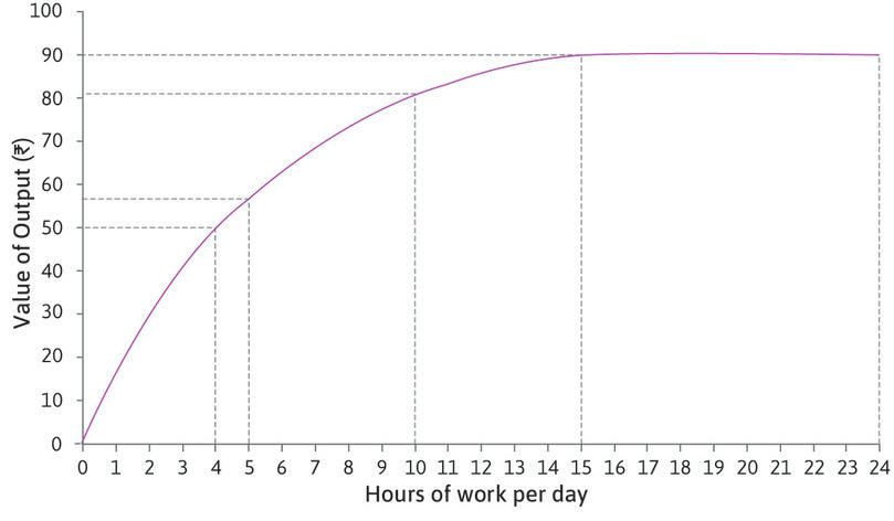
If we plot this relationship on a graph we get the curve in Figure 3.7. Sakina can obtain more output by working more, so the curve slopes upward. At 15 hours of work per day she gets the highest income she is capable of, which is Rs. 90. Any time spent working beyond that does not affect her output (she will be so tired that even working more she is not able to finish any more embroidering), and the curve becomes flat.
- average product
- Total output divided by a particular input, for example per worker (divided by the number of workers) or per worker per hour (total output divided by the total number of hours of labour put in).
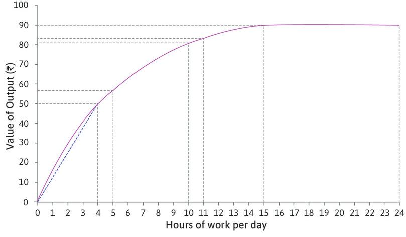
We can calculate Sakina’s average product of labour, as we did for the farmers in Unit 2. If she works for 4 hours per day she produces output worth Rs. 50. The average product—the average output per hour of work—is 50/4=Rs. 12.5. In Figure 3.7 it is the slope of a ray from the origin to the curve at 4 hours per day:
\[slope={\text{vertical axis} \over \text{horizontal axis}}=\frac{50}{4} = 12.5\]- marginal product
- The additional amount of output that is produced if a particular input was increased by one unit, while holding all other inputs constant.
Sakina’s marginal product is the increase in her output from increasing work by one hour. Follow the steps in Figure 3.7 to see how to calculate the marginal product, and compare it with the average product.
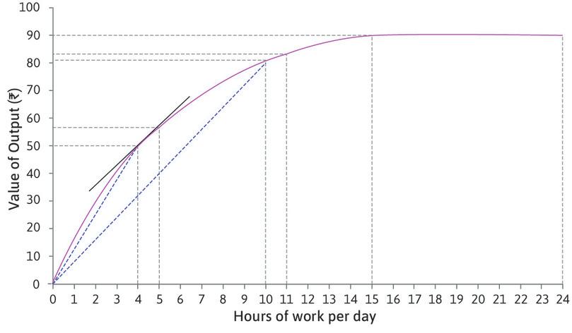
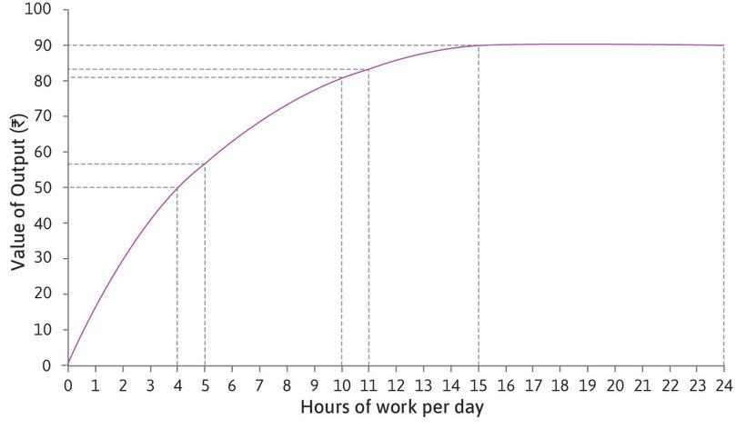
Figure 3.7 How does the amount of time spent working affect Sakina’s output?
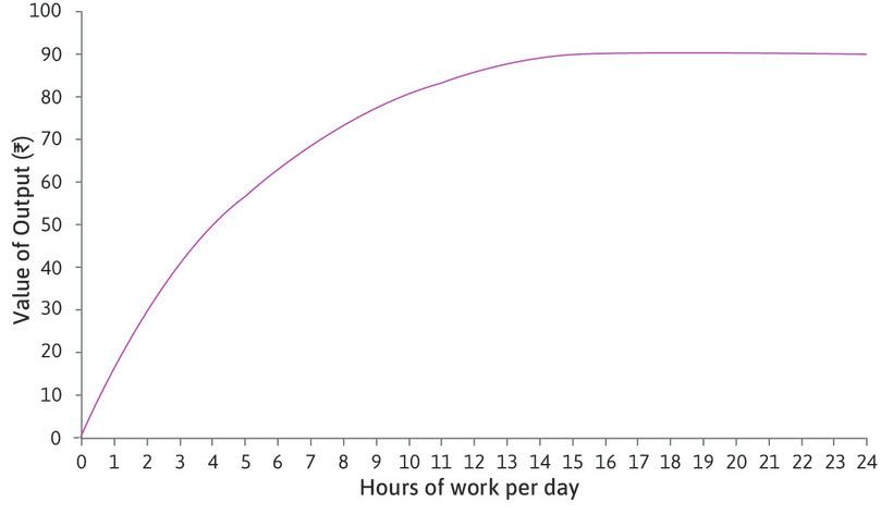
Sakina’s production function
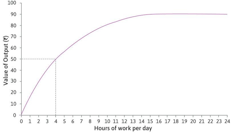
Four hours of work per day
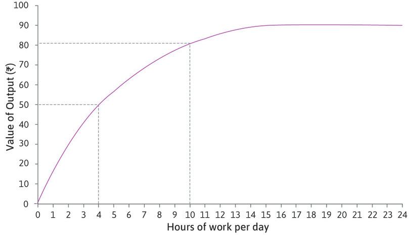
Ten hours of work per day

Sakina’s maximum output
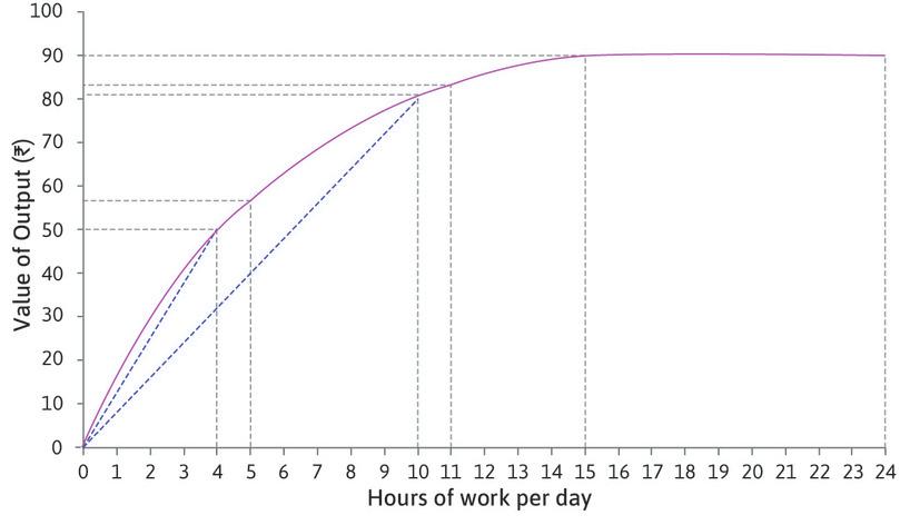
Increasing work time from 4 to 5 hours
Increasing work time from 10 to 11 hours
The average product of an hour spent working
The marginal product is lower than the average product
The marginal product is the slope of the tangent
At each point on the production function, the marginal product is the increase in the value of output from working one more hour. The marginal product corresponds to the slope of the production function.
Leibniz: Average and marginal productivity
- diminishing returns
- A situation in which the use of an additional unit of a factor of production results in a smaller increase in output than the previous increase. Also known as: diminishing marginal returns in production
Sakina’s production function in Figure 3.7 becomes flatter, the more hours she works so the marginal product of an additional hour falls as we move along the curve. The marginal product is diminishing. The model captures the idea that an extra hour of work helps a lot if you are not working much,but if you are already working a lot, then working even more does not help very much.
Leibniz: Diminishing marginal productivity
If we compare the marginal and average products at any point on Sakina’s production function, we find that the marginal product is below the average product. For example, when she works for four hours her average product is 50/4=12.5 rupees per hour, but an extra hour’s work raises the value of output from 50 to 57, so the marginal product is Rs. 7. This happens because the marginal product is diminishing: each hour is less productive than the ones that came before. And it implies that the average product is also diminishing: each additional hour of work per day lowers the average product of all her work time, taken as a whole.
This is another example of the diminishing average product of labour that we saw in Unit 2. In that case, the average product of labour in food production (the food produced per farmer) fell as more farmers cultivated a fixed area of land.
Lastly, notice that if Sakina was already working for 15 hours a day, the marginal product of an additional hour would be zero. Working more would not improve her output. As you might know from experience, a lack of either sleep or time to relax could even lower Sakina’s output if she worked more than 15 hours a day. If this were the case then her production function would start to slope downward, and Sakina’s marginal product would become negative.
Leibniz: Concave and convex functions
- tangency
- When two curves share one point in common but do not cross. The tangent to a curve at a given point is a straight line that touches the curve at that point but does not cross it.
Marginal change is an important and common concept in economics. You will often see it marked as a slope on a diagram. With a production function like the one in Figure 3.7, the slope changes continuously as we move along the curve. We have said that when Sakina works for four hours a day the marginal product is Rs. 7, the increase in the output from one more hour of work. Because the slope of the curve changes between 4 and 5 hours on the horizontal axis, this is only an approximation to the actual marginal product. More precisely, the marginal product is the rate at which the income increases, per hour of additional work. In Figure 3.7 the true marginal product is the slope of the tangent to the curve at 4 hours. In this unit we will use approximations so that we can work in whole numbers, but you may notice that sometimes these numbers are not quite the same as the slopes.
Exercise 3.2 Production functions
- Draw a graph to show a production function that, unlike Sakina’s, becomes steeper as the input increases.
- Can you think of an example of a production process that might have this shape? Why would the slope get steeper?
- What can you say about the marginal and average products in this case?
Question 3.3 Choose the correct answer(s)
Figure 3.7 shows Sakina’s production function, with the final income (the output) related to the number of hours spent working (the input).
Which of the following is true?
- Because there are no previous hours to consider, the average product for the initial hour is just the increase produced by a single hour, which in turn approximates to the marginal product from 0 to 1 hours (the precise marginal product changes over this interval, reflected in the decreasing slope of the production function).
- The marginal product is constant beyond 15 hours, but the average product continues to diminish. This is because the marginal product (zero) is less than the average product, which remains positive but is decreasing (more hours with no additional improvement reduces the average).
- If working for more than 15 hours had a negative effect on Sakina’s income, then the marginal product would be negative, implying a downward-sloping curve beyond 15 hours.
- The average product at 20 hours is 90/ 20 hours = 4.5 per hour. The marginal product, however, is zero—as indicated by the production function being flat beyond 15 hours.
3.3 Preferences
- preferences
- A description of the benefit or cost we associate with each possible outcome.
If Sakina has the production function shown in Figure 3.7, how many hours per day will she choose to work? The decision depends on her preferences—the things that she cares about. It is here that people and cultures differ. Let us assume that Sakina sells the output for its value. For example, if she produces Rs. 90 worth of cloth, she is able to sell it all, and that is her income. If Sakina cared only about the things she could buy with her income, she should work for 15 hours a day. But, like other people, Sakina also cares about her time, her relationships—she needs to take care of the children, to cook and would like to go out or watch TV. So she faces a trade-off: how much income is she willing to give up in order to spend time on things other than embroidery work? Work (in the sense of exerting effort to accomplish something) is not intrinsically unpleasant; people sometimes enjoy working hard and Sakina may too. But work does involve trade-offs, and working more necessarily means less time for doing things that you otherwise want to, even if you enjoy your job.
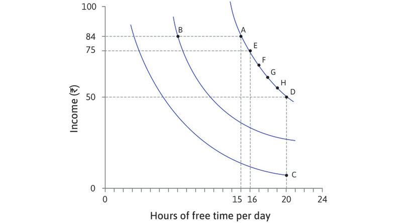
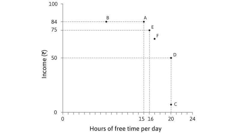
We illustrate her preferences using Figure 3.8, with time spent on other activities on the horizontal axis and final income on the vertical axis. Free time is defined as all the time that she does not spend working. Every point in the diagram represents a different combination of free time and final income. Given her production function, not every combination that Sakina would want will be possible, but for the moment we will only consider the combinations that she would prefer.
We can assume:
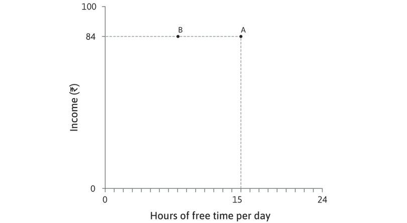
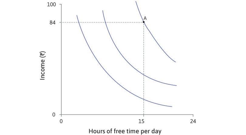
- For a given income, she prefers a combination with more time for other things than paid work to one with less time. Therefore, even though both A and B in Figure 3.6 correspond to an income of 84, Sakina prefers A because it gives her more free time.
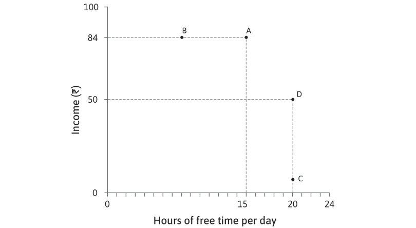
- Similarly, if two combinations both have 20 hours of time outside paid work, she prefers the one with a higher income.
- But compare points A and D in the table. Would Sakina prefer D (low income, plenty of free time) or A (higher income, less free time)? One way to find out would be to ask her.
- utility
- A numerical indicator of the value that one places on an outcome, such that higher valued outcomes will be chosen over lower valued ones when both are feasible.
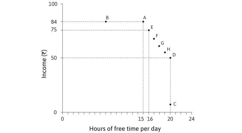
Suppose she says she is indifferent between A and D, meaning she would feel equally satisfied with either outcome. We say that these two outcomes would give Sakina the same utility. And we know that she prefers A to B, so B provides lower utility than A or D.
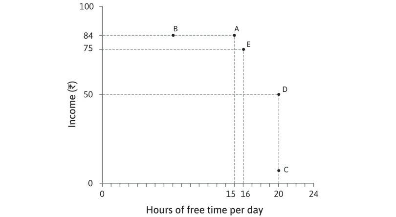
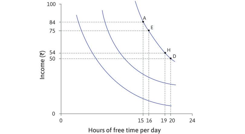
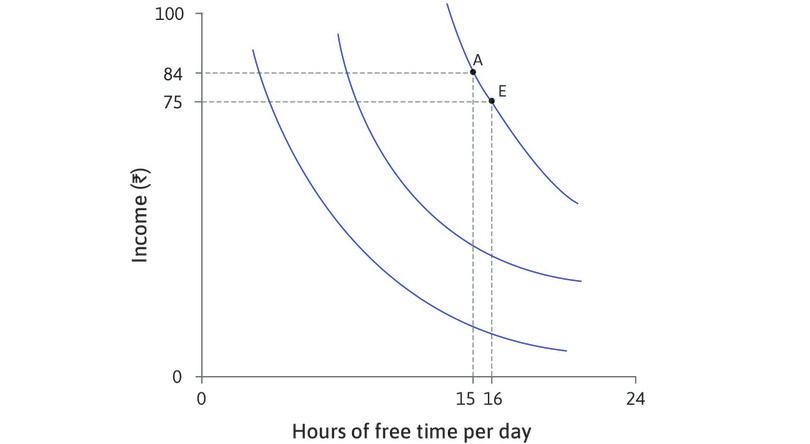
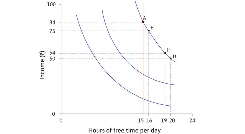
A systematic way to graph Sakina’s preferences would be to start by looking for all of the combinations that give her the same utility as A and D. We could ask Sakina another question: ‘Imagine that you could have the combination at A (15 hours of free time, Rs. 84). How many rupees would you be willing to sacrifice for an extra hour of free time?’ Suppose that after due consideration, she answers ‘nine’. Then we know that she is indifferent between A and E (16 hours, Rs. 75). Then we could ask the same question about combination E, and so on until point D. Eventually we could draw up a table like the one in Figure 3.6. Sakina is indifferent between A and E, between E and F, and so on, which means she is indifferent between all of the combinations from A to D.
- indifference curve
- A curve of the points which indicate the combinations of goods that provide a given level of utility to the individual.
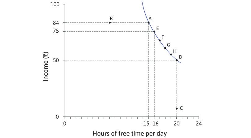
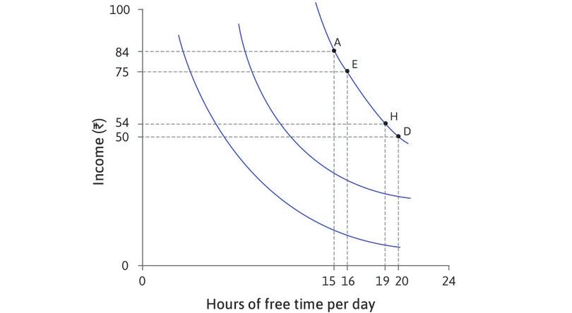
The combinations in the table are plotted in Figure 3.8, and joined together to form a downward-sloping curve, called an indifference curve, which joins together all of the combinations that provide equal utility or ‘satisfaction’.
| A | E | F | G | H | D | |
|---|---|---|---|---|---|---|
| Hours of free time | 15 | 16 | 17 | 18 | 19 | 20 |
| Income (Rs.) | 84 | 75 | 67 | 60 | 54 | 50 |
Figure 3.8 Mapping Sakina’s preferences.
| A | E | F | G | H | D | |
|---|---|---|---|---|---|---|
| Hours of free time | 15 | 16 | 17 | 18 | 19 | 20 |
| Income (Rs.) | 84 | 75 | 67 | 60 | 54 | 50 |
Sakina prefers more free time to less free time
| A | E | F | G | H | D | |
|---|---|---|---|---|---|---|
| Hours of free time | 15 | 16 | 17 | 18 | 19 | 20 |
| Income (Rs.) | 84 | 75 | 67 | 60 | 54 | 50 |
Sakina prefers a high income to a low income
| A | E | F | G | H | D | |
|---|---|---|---|---|---|---|
| Hours of free time | 15 | 16 | 17 | 18 | 19 | 20 |
| Income (Rs.) | 84 | 75 | 67 | 60 | 54 | 50 |
Indifference
| A | E | F | G | H | D | |
|---|---|---|---|---|---|---|
| Hours of free time | 15 | 16 | 17 | 18 | 19 | 20 |
| Income (Rs.) | 84 | 75 | 67 | 60 | 54 | 50 |
More combinations giving the same utility
| A | E | F | G | H | D | |
|---|---|---|---|---|---|---|
| Hours of free time | 15 | 16 | 17 | 18 | 19 | 20 |
| Income (Rs.) | 84 | 75 | 67 | 60 | 54 | 50 |
Constructing the indifference curve
| A | E | F | G | H | D | |
|---|---|---|---|---|---|---|
| Hours of free time | 15 | 16 | 17 | 18 | 19 | 20 |
| Income (Rs.) | 84 | 75 | 67 | 60 | 54 | 50 |
Constructing the indifference curve
| A | E | F | G | H | D | |
|---|---|---|---|---|---|---|
| Hours of free time | 15 | 16 | 17 | 18 | 19 | 20 |
| Income (Rs.) | 84 | 75 | 67 | 60 | 54 | 50 |
Other indifference curves
If you look at the three curves drawn in Figure 3.8, you can see that the one through A gives higher utility than the one through B. The curve through C gives the lowest utility of the three. To describe preferences we don’t need to know the exact utility of each option; we only need to know which combinations provide more or less utility than others.
- consumption good
- A good or service that satisfies the needs of consumers over a short period.
The curves we have drawn capture our typical assumptions about people’s preferences between two goods. In other models, these will often be consumption goods such as food or clothing, and we refer to the person as a consumer. In our model of a textile worker’s preferences, the goods are ‘final income’ and ‘free time’. Notice that:
- Indifference curves slope downward due to trade-offs: If you are indifferent between two combinations, the combination that has more of one good must have less of the other good.
- Higher indifference curves correspond to higher utility levels: As we move up and to the right in the diagram, further away from the origin, we move to combinations with more of both goods.
- Indifference curves are usually smooth: Small changes in the amounts of goods don’t cause big jumps in utility.
- Indifference curves do not cross: Why? See Exercise 3.3.
- As you move to the right along an indifference curve, it becomes flatter.
- marginal rate of substitution (MRS)
- The trade-off that a person is willing to make between two goods. At any point, this is the slope of the indifference curve. See also: marginal rate of transformation.
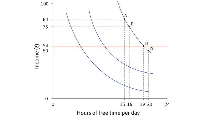
To understand the last property in the list, look at Sakina’s indifference curves, which are plotted again in Figure 3.9. If she is at A, with 15 hours of free time and an income of 84, she would be willing to sacrifice 9 rupees for an extra hour of free time, taking her to E (remember that she is indifferent between A and E). We say that her marginal rate of substitution (MRS) between income and free time at A is nine; it is the reduction in her income that would keep Sakina’s utility constant following a one-hour increase of free time.
We have drawn the indifference curves as becoming gradually flatter because it seems reasonable to assume that the more free time and the lower the income she has, the less willing she will be to sacrifice further percentage points in return for free time, so her MRS will be lower. In Figure 3.9 we have calculated the MRS at each combination along the indifference curve. You can see that, when Sakina has more free time and a lower income, the MRS—the number of percentage points she would give up to get an extra hour of free time—gradually falls.
| A | E | F | G | H | D | |||||||
|---|---|---|---|---|---|---|---|---|---|---|---|---|
| Hours of free time | 15 | 16 | 17 | 18 | 19 | 20 | ||||||
| Income | 84 | 75 | 67 | 60 | 54 | 50 | ||||||
| Marginal rate of substitution between income and free time | 9 | 8 | 7 | 6 | 4 | |||||||
Figure 3.9 The marginal rate of substitution.
Sakina’s indifference curves
Point A
Sakina is indifferent between A and E
Sakina is indifferent between H and D
All combinations with 15 hours of free time
All combinations with an income of 54
The MRS is just the slope of the indifference curve, and it falls as we move to the right along the curve. If you think about moving from one point to another in Figure 3.9 you can see that the indifference curves get flatter if you increase the amount of free time, and steeper if you increase the income. When free time is scarce relative to income, Sakina is less willing to sacrifice an hour for a higher income: her MRS is high and her indifference curve is steep.
As the analysis in Figure 3.9 shows, if you move up the vertical line through 15 hours, the indifference curves get steeper: the MRS increases. For a given amount of free time, Sakina is willing to give up more income for an additional hour when she has (relatively) a lot of income compared to when she has very little. By the time you reach A, where her income is 84, the MRS is high; income is large enough here that she is willing to give up 9 rupees for an extra hour of free time.
Leibniz: Indifference curves and the marginal rate of substitution
You can see the same effect if you fix the income and vary the amount of free time. If you move to the right along the horizontal line for an income of 54, the MRS becomes lower at each indifference curve. As free time becomes more plentiful, Sakina becomes less and less willing to give up income points for more time.
Exercise 3.3 Why indifference curves never cross
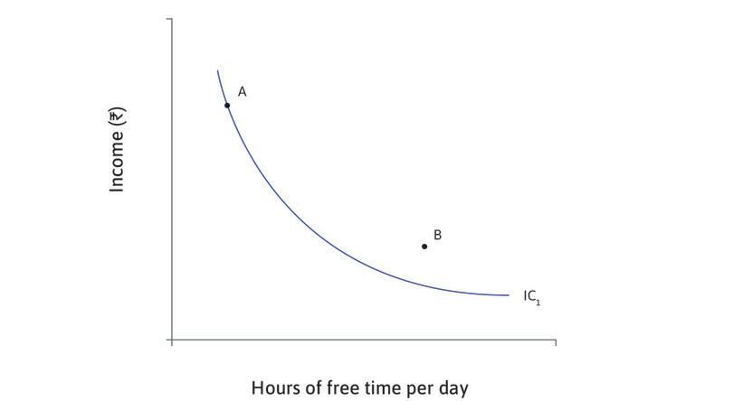
In the diagram below, IC1 is an indifference curve joining all the combinations that give the same level of utility as A. Combination B is not on IC1.
![]()
- Does combination B give higher or lower utility than combination A? How do you know?
- Draw a sketch of the diagram, and add another indifference curve, IC2, that goes through B and crosses IC1. Label the point at which they cross as C.
- Combinations B and C are both on IC2. What does that imply about their levels of utility?
- Combinations C and A are both on IC1. What does that imply about their levels of utility?
- According to your answers to (3) and (4), how do the levels of utility at combinations A and B compare?
- Now compare your answers to (1) and (5), and explain how you know that indifference curves can never cross.
Exercise 3.4 Your marginal rate of substitution
Imagine that you are offered a job at the end of your university course with a salary per hour (after taxes) of Rs. 400. Your future employer then says that you will work for 40 hours per week leaving you with 128 hours of free time per week. You tell a friend: ‘at that wage, 40 hours is exactly what I would like.’
- Draw a diagram with free time on the horizontal axis and weekly pay on the vertical axis, and plot the combination of hours and the wage corresponding to your job offer, calling it A. Assume you need about 10 hours a day for sleeping and eating, so you may want to draw the horizontal axis with 70 hours at the origin.
- Now draw an indifference curve so that A represents the hours you would have chosen yourself.
- Now imagine you were offered another job requiring 45 hours of work per week. Use the indifference curve you have drawn to estimate the level of weekly pay that would make you indifferent between this and the original offer.
- Do the same for another job requiring 35 hours of work per week. What level of weekly pay would make you indifferent between this and the original offer?
- Use your diagram to estimate your marginal rate of substitution between pay and free time at A.
Question 3.4 Choose the correct answer(s)
Figure 3.8 shows Sakina’s indifference curves for non-work time and final income. Which of the following is true?
- The indifference curve through C is lower than that through B. Hence Sakina prefers B to C.
- A, where Sakina has the income of 84 and 15 hours of non-work time, and D, where Sakina has the income of 50 with 20 hours of non-work time, are on the same indifference curve.
- At D Sakina has the same amount of non-work time but a higher income.
- The opposite trade-off is true: going from G to D, Sakina is willing to give up 10 rupees of income for 2 extra hours of non work time. Going from G to E, she is willing to give up 2 hours of non-work time for 15 extra rupees of income.
Question 3.5 Choose the correct answer(s)
What is the marginal rate of substitution (MRS)?
- The marginal rate of substitution represents the ratio of the trade-off at the margin, in other words, how much of one good the consumer is willing to sacrifice for one extra unit of the other.
- This is the definition of the marginal rate of substitution.
- The MRS is the amount of one good that can be substituted for one unit of the other while keeping utility constant.
- The slope of the indifference curve represents the marginal rate of substitution: the trade-off between two goods that keeps utility constant.
3.4 Opportunity costs
- opportunity cost
- When taking an action implies forgoing the next best alternative action, this is the net benefit of the foregone alternative.
Sakina faces a dilemma: we know from looking at her preferences that she wants both her income and her free time to be as high as possible. But given her production function, she cannot increase her free time without getting a lower income. Another way of expressing this is to say that free time has an opportunity cost: to get more free time, Sakina has to forgo the opportunity of getting a higher income.
In economics, opportunity costs are relevant whenever we study individuals choosing between alternative and mutually exclusive courses of action. In Unit 2 we evaluated a course of action A by comparing it with the ‘next best alternative’ action B. When we consider the cost of taking action A we include the fact that if we do A, we cannot do B. So ‘not doing B’ becomes part of the cost of doing A. This is called an opportunity cost because doing A means forgoing the opportunity to do B.
Imagine that an accountant and an economist have been asked to report the cost of going to a concert, A, in a theatre, which has a Rs. 500 admission cost. In a nearby park there is concert B, which is free but happens at the same time.
- Accountant
- The cost of concert A is your ‘out-of-pocket’ cost: you paid Rs. 500 for a ticket, so the cost is Rs. 500.
- Economist
- But what do you have to give up to go to concert A? You give up Rs. 500, plus the enjoyment of the free concert in the park. So the cost of concert A for you is the out-of-pocket cost plus the opportunity cost.
Suppose that the most you would have been willing to pay to attend the free concert in the park (if it wasn’t free) was Rs. 300. The benefit of your next best alternative to concert A would be Rs. 300 of enjoyment in the park. This is the opportunity cost of going to concert A.
- economic cost
- The out-of-pocket cost of an action, plus the opportunity cost.
So the total economic cost of concert A is Rs. 500 + Rs. 300 = Rs. 800. If the pleasure you anticipate from being at concert A is greater than the economic cost, say Rs. 1,000, then you will forego concert B and buy a ticket to the theatre. On the other hand, if you anticipate Rs. 700 worth of pleasure from concert A, then the economic cost of Rs. 800 means you will not choose to go to the theatre. In simple terms, given that you have to pay Rs. 500 for the ticket, you will instead opt for concert B, pocketing the Rs. 500 to spend on other things and enjoying Rs. 300 worth of benefit from the free park concert.
Why don’t accountants think this way? Because it is not their job. Accountants are paid to keep track of money, not to provide decision rules on how to choose among alternatives, some of which do not have a stated price. But making sensible decisions and predicting how sensible people will make decisions involve more than keeping track of money. An accountant might argue that the park concert is irrelevant:
- Accountant
- Whether or not there is a free park concert does not affect the cost of going to the concert A. The cost to you is always Rs. 500.
- Economist
- But whether or not there is a free park concert can affect whether you go to concert A or not, because it changes your available options. If your enjoyment from A is Rs. 700 and your next best alternative is staying at home, with enjoyment of Rs. 0, you will choose concert A. However, if concert B is available, you will choose it over A.
- economic rent
- A payment or other benefit received above and beyond what the individual would have received in his or her next best alternative (or reservation option). See also: reservation option.
In Unit 2, we said that if an action brings greater net benefits than the next best alternative, it yields an economic rent and you will do it. Another way of saying this is that you receive an economic rent from taking an action when it results in a benefit greater than its economic cost (the sum of out-of-pocket and opportunity costs).
The table in Figure 3.10 summarizes the example of your choice of which concert to attend.
| A high value on the theatre choice (A) | A low value on the theatre choice (A) | |
|---|---|---|
| Out-of-pocket cost (price of ticket for A) | Rs. 500 | Rs. 500 |
| Opportunity cost (foregone pleasure of B, park concert) | Rs. 300 | Rs. 300 |
| Economic cost (sum of out-of-pocket and opportunity cost) | Rs. 800 | Rs. 800 |
| Enjoyment of theatre concert (A) | Rs. 1,000 | Rs. 700 |
| Economic rent (enjoyment minus economic cost) | Rs. 200 | Rs. −100 |
| Decision | A: Go to the theatre concert. | B: Go to the park concert. |
Figure 3.10 Opportunity costs and economic rent: Which concert will you choose?
Question 3.6 Choose the correct answer(s)
You are a bus driver in Bengaluru who earns Rs. 500 for a day’s work. You have been offered a movie ticket starring your favourite movie star for Rs. 400. As a film buff, you value the experience at Rs. 1000. With this information, what can we say?
- By going to the movie you are foregoing the opportunity of earning Rs. 500 from bus driving. This is your opportunity cost.
- The economic cost is the sum of the actual price you pay plus the opportunity cost, which in this case is Rs. 400 + Rs. 500 = Rs. 900.
- The economic rent of an action is its benefit minus its economic cost (out-of-pocket plus opportunity costs). Therefore, the economic rent is Rs. 1000 – Rs. 400 – Rs. 500 = Rs. 100.
- The maximum price you would have paid for the movie ticket is the price at which your economic rent would be zero, which in this case is Rs. 500.
Exercise 3.5 Opportunity costs
The British government introduced legislation in 2012 that gave universities the option to raise their tuition fees. Most chose to increase annual tuition fees for students from £3,000 to £9,000.
Does this mean that the cost of going to university has tripled? (Think about how an accountant and an economist might answer this question. To simplify, assume that the tuition fee is an ‘out of pocket’ cost. Ignore student loans.)
3.5 The feasible set
Now we return to Sakina’s problem of how to choose between income and free time. Free time has an opportunity cost in the form of lost income (equivalently, we might say that income has an opportunity cost in the form of the free time Sakina has to give up to obtain it). But before we can describe how Sakina resolves her dilemma, we need to work out precisely which alternatives are available to her.
To answer this question, we look again at the production function. In Figure 3.7, we modelled the production function as a relationship translating Sakina’s hours of work into output (units of cloth). However, we also assumed a little later that she is able to sell all the cloth for its value. So now, her value of output and final income are the same, and both terms can be used interchangeably.
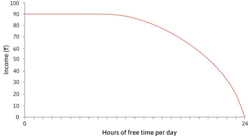
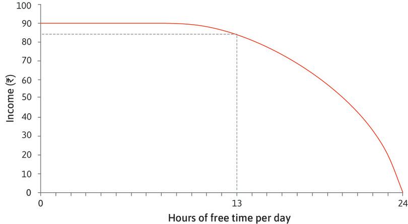
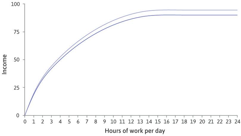
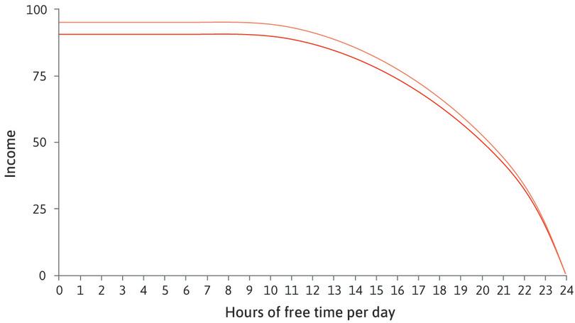
This time we will show how the final income depends on the amount of free time, rather than work time. There are 24 hours in a day. Sakina must divide this time between working (all the hours devoted to embroidering) and free time (all the rest of her time). Figure 3.11 shows the relationship between her final income and hours of free time per day—the mirror image of Figure 3.7. If Sakina works solidly for 24 hours, that means zero hours of free time and a final income of 90. If she chooses 24 hours of free time per day (i.e., she does not work for pay), we assume she will get an income of zero.
- feasible frontier
- The curve made of points that defines the maximum feasible quantity of one good for a given quantity of the other. See also: feasible set.
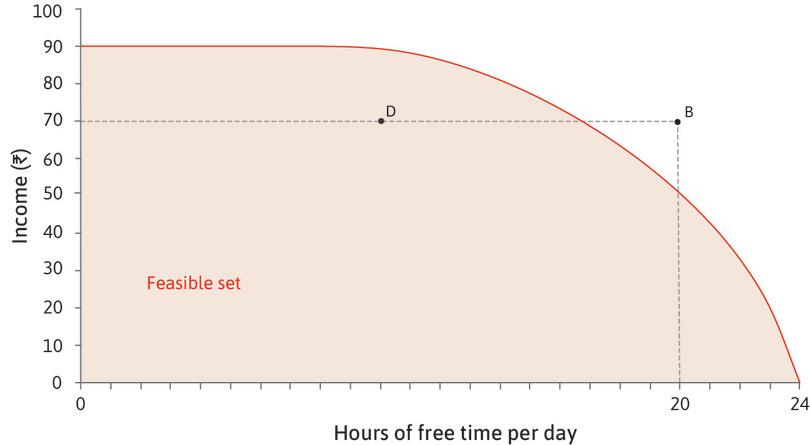
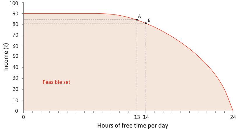
In Figure 3.11, the axes are income and free time, the two goods that give Sakina utility. If we think of her choosing to consume a combination of these two goods, the curved line in Figure 3.11 shows what is feasible. It represents her feasible frontier: the highest income she can achieve given the amount of free time she wants.
- feasible set
- All of the combinations of the things under consideration that a decision-maker could choose given the economic, physical or other constraints that he faces. See also: feasible frontier.
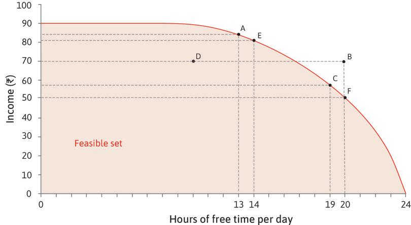
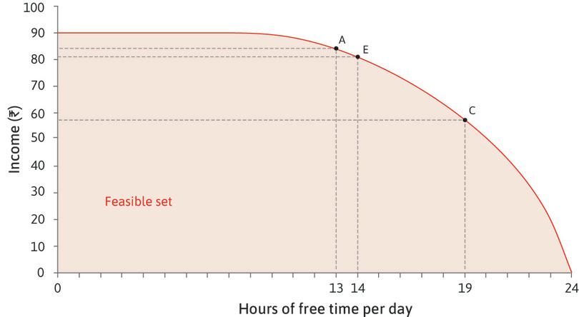
| A | E | C | F | |
|---|---|---|---|---|
| Free time | 13 | 14 | 19 | 20 |
| Income | 84 | 81 | 57 | 50 |
| Opportunity cost | 3 | 7 |
Figure 3.11 How does Sakina’s choice of free time affect her income?
The feasible frontier
A feasible combination
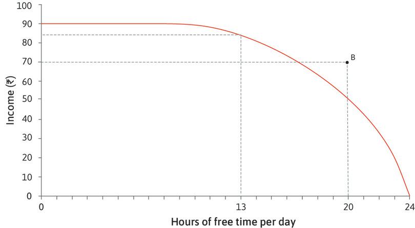
Infeasible combinations
A feasible combination
Inside the frontier
The feasible set
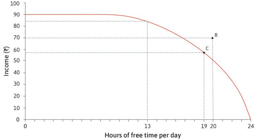
The opportunity cost of free time
The opportunity cost varies
The slope of the feasible frontier
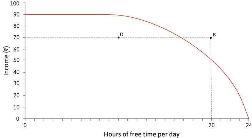
Any combination of free time and income that is on or inside the frontier is feasible. Combinations outside the feasible frontier are said to be infeasible given Sakina’s abilities and conditions of work. On the other hand, even though a combination lying inside the frontier is feasible, choosing it would imply Sakina has effectively thrown away something that she values. If she worked for 14 hours a day, then according to our model, she could guarantee herself an income of Rs. 89. But she could obtain a lower income (Rs. 70, say), if she just stopped working hard throughout the hour. It would be foolish to throw away income like this for no reason, but it would be possible.
By choosing a combination inside the frontier, Sakina would be giving up something that is freely available—something that has no opportunity cost. She could obtain a higher income without sacrificing any free time, or have more time without reducing her income.
The feasible frontier is a constraint on Sakina’s choices. It represents the trade-off she must make between income and free time. At any point on the frontier, taking more free time has an opportunity cost in terms of income points foregone, corresponding to the slope of the frontier.
- marginal rate of transformation (MRT)
- The quantity of some good that must be sacrificed to acquire one additional unit of another good. At any point, it is the slope of the feasible frontier. See also: marginal rate of substitution.
Another way to express the same idea is to say that the feasible frontier shows the marginal rate of transformation (MRT): the rate at which Sakina can transform free time into income points. Look back at Figure 3.11 at the slope of the frontier between points A and E:
- The slope of AE (vertical distance divided by horizontal distance) is −3.
- At point A, Sakina could get one more unit of free time by giving up 3 rupees of income. The opportunity cost of a unit of free time is 3.
- At point E, Sakina could transform one unit of time into 3 rupees of income. The marginal rate at which she can transform free time into income is 3.
Note that the slope of AE is only an approximation to the slope of the frontier. More precisely, the slope at any point is the slope of the tangent, and this represents both the MRT and the opportunity cost at that point.
Note that we have now identified two trade-offs:
Leibniz: Marginal rates of transformation and substitution
- The marginal rate of substitution (MRS): In the previous section, we saw that it measures the trade-off that Sakina is willing to make between income and free time.
- The marginal rate of transformation (MRT): In contrast, this measures the trade-off that Sakina is constrained to make by the feasible frontier.
As we shall see in the next section, the choice Sakina makes between her income and her free time will strike a balance between these two trade-offs.
Question 3.7 Choose the correct answer(s)
Look at Figure 3.7 which shows Sakina’s production function: how the final income (the output) depends on the number of hours spent working (the input).
Free time per day is given by 24 hours minus the hours of work per day. Consider Sakina’s feasible set of combinations of final income and hours of free time per day. What can we conclude?
- The hours of free time per day is already given as 24 hours minus the hours of work per day. Therefore, the number of hours spent sleeping is included in the hours of free time.
- Given that the production function is just the feasible frontier except that it takes negative free time (hours of study) as its input, the former is simply the latter mirrored across the horizontal axis and shifted horizontally.
- The production function is horizontal after 15 hours of work per day. Therefore, the feasible frontier is horizontal only up to 9 hours of free time per day.
- 10 hours of study is equivalent to 14 hours of free time given a 24-hour day, and the marginal product of labour (additional output per labour hour) is the same as the marginal rate of transformation (trade-off between extra output and labour), so these two values are equal.
3.6 Decision making and scarcity
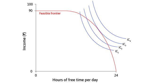
The final step in this decision-making process is to determine the combination of income and free time that Sakina will choose. Figure 3.12a brings together her feasible frontier (Figure 3.11) and indifference curves (Figure 3.8). Recall that the indifference curves indicate what Sakina prefers, and their slopes shows the trade-offs that she is willing to make; the feasible frontier is the constraint on her choice, and its slope shows the trade-off she is constrained to make.
Figure 3.12a shows four indifference curves, labelled IC1 to IC4. IC4 represents the highest level of utility because it is the furthest away from the origin. However, no combination of income and free time on IC4 is feasible, however, because the whole indifference curve lies outside the feasible set. Suppose that Sakina considers choosing a combination somewhere in the feasible set, on IC1. By working through the steps in Figure 3.12a, you will see that she can increase her utility by moving to points on higher indifference curves until she reaches a feasible choice that maximizes her utility.
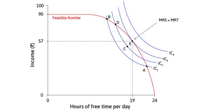
Figure 3.12a How many hours does Sakina decide to work?
Which point will Sakina choose?

Feasible combinations

Could do better
Could do better
The best feasible trade-off
The best feasible trade-off
MRS = MRT
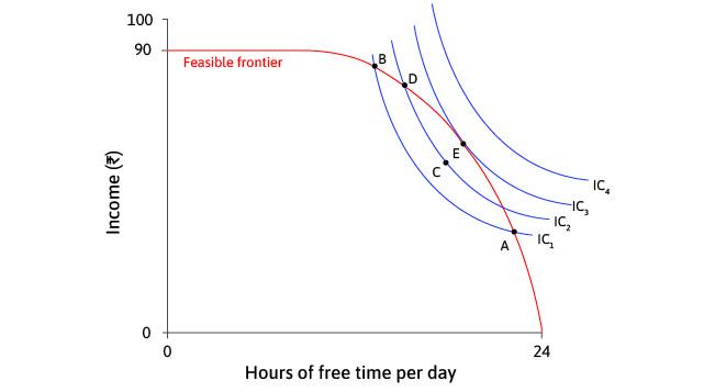
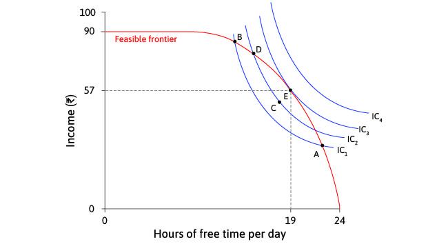
Sakina maximises her utility at point E, at which her indifference curve is tangent to the feasible frontier. The model predicts that Sakina will:
- Choose to spend 5 hours each day working, and 19 hours on other activities
- Obtain an income of Rs. 57 as a result
We can see from Figure 3.12a that at E, the feasible frontier and the highest attainable indifference curve IC3 are tangent to each other (they touch but do not cross). At E, the slope of the indifference curve is the same as the slope of the feasible frontier. Now, remember that the slopes represent the two trade-offs facing Sakina:
- The slope of the indifference curve is the MRS: It is the trade-off she is willing to make between free time and income.
- The slope of the frontier is the MRT: It is the trade-off that she is constrained to make between free time and income because it is not possible to go beyond the feasible frontier.
Sakina achieves the highest possible utility where the two trade-offs just balance (E). Her optimal combination of income and free time is at the point where the marginal rate of transformation is equal to the marginal rate of substitution.
Leibniz: Optimal allocation of free time: MRT meets MRS
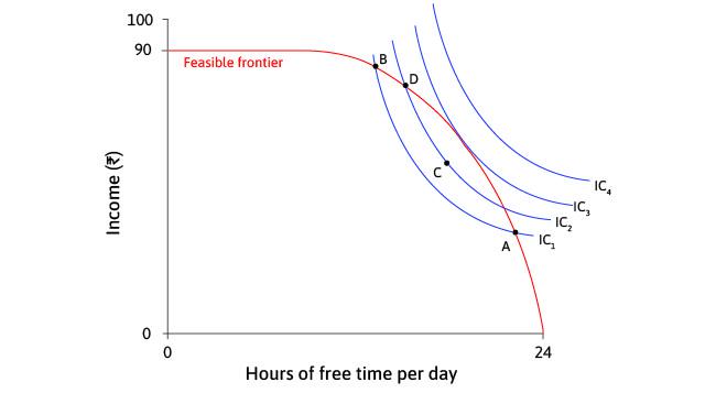
Figure 3.12b shows the MRS (slope of indifference curve) and MRT (slope of feasible frontier) at the points shown in Figure 3.12a. At B and D, the amount of income Sakina is willing to trade for an hour of free time (MRS) is greater than the opportunity cost of that hour (MRT), so she prefers to increase her free time. At A, the MRT is greater than the MRS so she prefers to decrease her free time. And, as expected, at E the MRS and MRT are equal.
| B | D | E | A | |
|---|---|---|---|---|
| Free time (hours) | 13 | 15 | 19 | 22 |
| Income (Rs.) | 84 | 78 | 57 | 33 |
| MRT | 2 | 4 | 7 | 9 |
| MRS | 20 | 15 | 7 | 3 |
Figure 3.12b How many hours does Sakina decide to work?
- constrained choice problem
- This problem is about how we can do the best for ourselves, given our preferences and constraints, and when the things we value are scarce. See also: constrained optimization problem.
We have modelled the worker’s decision on work hours as what we call a constrained choice problem: a decision-maker (Sakina) pursues an objective (utility maximization in this case) subject to a constraint (her feasible frontier).
In our example, both free time and income are scarce for Sakina because:
- Free time and income are goods: Sakina values both of them.
- Each has an opportunity cost: More of one good means less of the other.
In constrained choice problems, the solution is the individual’s optimal choice. If we assume that utility maximization is Sakina’s goal, the optimal combination of income and free time is a point on the feasible frontier at which:
\[\text{MRS = MRT}\]The table in Figure 3.13 summarizes Sakina’s trade-offs.
| The trade-off | Where it is on the diagram | It is equal to … | |
|---|---|---|---|
| MRS | Marginal rate of substitution: The amount of income Sakina is willing to trade for an hour of free time | The slope of the indifference curve | |
| MRT, or opportunity cost of free time | Marginal rate of transformation: The amount of income Sakina would gain (or lose) by giving up (or taking) another hour of free time | The slope of the feasible frontier | The marginal product of labour |
Figure 3.13 Sakina’s trade-offs.
Exercise 3.6 Exploring scarcity
Describe a situation in which Sakina’s income and free time would not be scarce. Remember, scarcity depends on both her preferences and the production function.
Question 3.8 Choose the correct answer(s)
Figure 3.12a shows Sakina’s feasible frontier and her indifference curves for final income and hours of free time per day. Suppose that all workers have the same feasible frontier, but their indifference curves may differ in shape and slope depending on their preferences.
Use the diagram to decide which of the following is (are) correct.
- If Sakina were at a point on the feasible frontier where MRS ≠ MRT, then she would be willing to give up more of one good than would actually be necessary to get some of the other. Therefore, she will choose to do so until she reaches a point where MRS = MRT.
- Along the feasible frontier, Sakina would be on a higher indifference curve at E than at D. Therefore point D is not the optimal choice.
- Workers with flatter indifference curves (more willing to sacrifice more hours of free time for the same number of extra income) have a lower marginal rate of substitution. Therefore, they will choose bundles to the left of E (such as D) where their indifference curves are tangent to the feasible frontier.
- The points along the feasible frontier to the left of E have higher ratios of final income per hour of free time, but are not optimal. The optimal point is where marginal rate of substitution equals marginal rate of transformation.
3.7 Hours of work and economic growth
In 1930, John Maynard Keynes, a British economist, published an essay entitled ‘Economic Possibilities for our Grandchildren’, in which he suggested that in the 100 years that would follow, technological improvement would make us, on average, about eight times better off.1 What he called ‘the economic problem, the struggle for subsistence’ would be solved, and we would not have to work more than, say, 15 hours per week to satisfy our economic needs. The question he raised was: how would we cope with all of the additional leisure time?
Keynes’ prediction for the rate of technological progress in countries such as the UK and the US has been approximately right, and working hours have indeed fallen, although much less than he expected—it seems unlikely that average working hours will be 15 hours per week by 2030. An article by Tim Harford in the Undercover Economist column of the Financial Times examines why Keynes’ prediction was wrong.2.
As we saw in Unit 2, new technologies raise the productivity of labour. We now have the tools to analyse the effects of increased productivity on living standards, specifically on incomes and the free time of workers.
To understand this, let us now apply our model of constrained choice to Angela, a self-sufficient grain farmer. We assume that Angela produces grain to eat and does not sell it to anyone else. If she produces too little grain, she will starve.
What is stopping her producing the most grain possible? Like Sakina, Angela also values free time—she gets utility from both free time and consuming grain.
But her choice is constrained: producing grain takes labour time, and each hour of labour means Angela foregoes an hour of free time. The hour of free time sacrificed is the opportunity cost of the grain produced. Like Sakina, Angela faces a problem of scarcity: she has to make a choice between her consumption of grain and her consumption of free time.
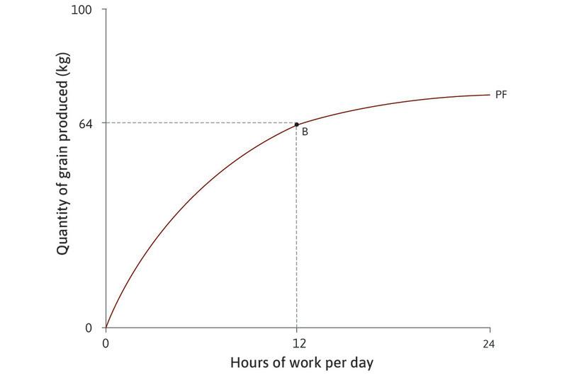
Figure 3.14 shows the initial production function before the change occurs: the relationship between the number of hours worked and the amount of grain produced. Notice that the graph has a similar concave shape to Sakina’s production function: the marginal product of an additional hour’s work, shown by the slope, diminishes as the number of hours increases.
A technological improvement such as seeds with a higher yield, or better equipment that makes harvesting quicker, will increase the amount of grain produced in a given number of hours. The analysis in Figure 3.14 demonstrates the effect on the production function.
| Working hours | 0 | 1 | 2 | 3 | 4 | 5 | 6 | 7 | 8 | 9 | 10 | 11 | 12 | 13 | 18 | 24 | |||||||
| Grain (kg) | 0 | 9 | 18 | 26 | 33 | 40 | 46 | 51 | 55 | 58 | 60 | 62 | 64 | 66 | 69 | 72 |
Figure 3.14 How technological change affects the production function.
| Working hours | 0 | 1 | 2 | 3 | 4 | 5 | 6 | 7 | 8 | 9 | 10 | 11 | 12 | 13 | 18 | 24 | |||||||
| Grain (kg) | 0 | 9 | 18 | 26 | 33 | 40 | 46 | 51 | 55 | 58 | 60 | 62 | 64 | 66 | 69 | 72 |
The initial technology
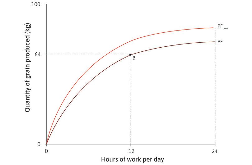
A technological improvement

More grain for the same amount of work
Or same grain, less work
Notice that the new production function is steeper than the original one for every given number of hours. The new technology has increased Angela’s marginal product of labour: at every point, an additional hour of work produces more grain than under the old technology.
Leibniz: Modelling technological change
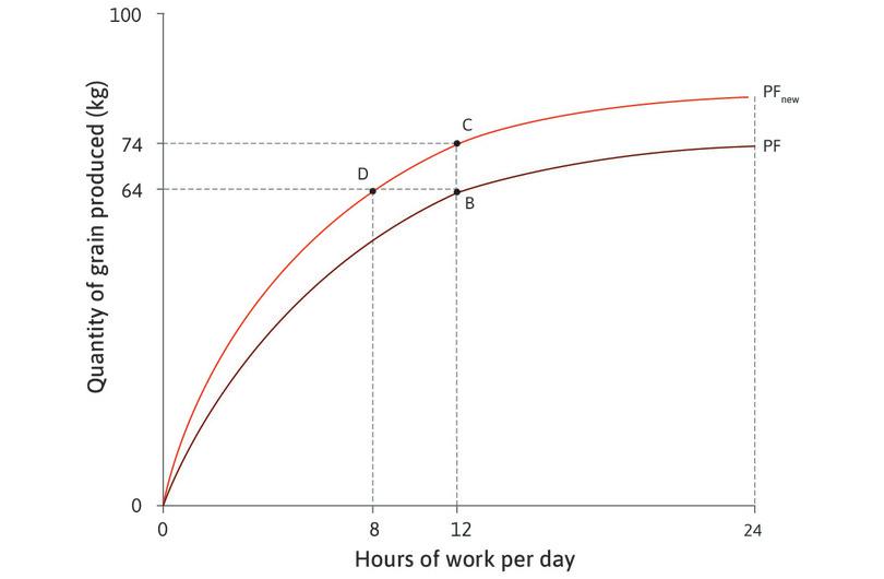
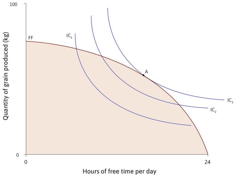
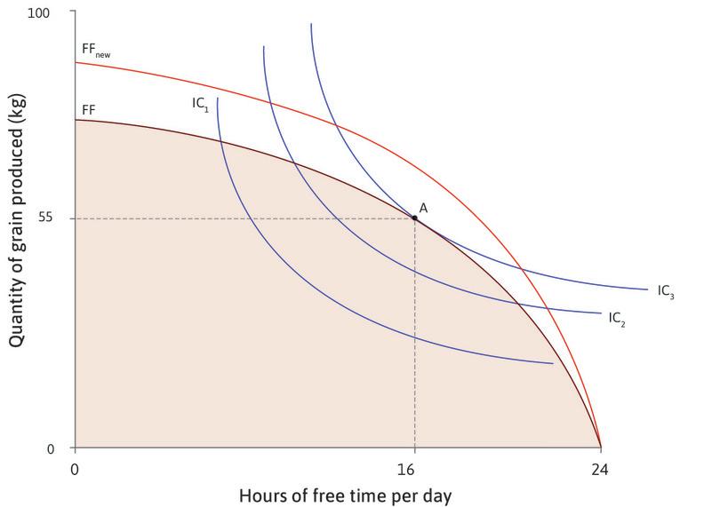
Figure 3.15 shows Angela’s feasible frontier, which is just the mirror image of the production function, for the original technology (FF), and the new one (FFnew).
As before, what we call free time is all of the time that is not spent working to produce grain—it includes time for eating, sleeping, and everything else that we don’t count as farm work, as well as her leisure time. The feasible frontier shows how much grain can be produced and consumed for each possible amount of free time. Points B, C, and D represent the same combinations of free time and grain as in Figure 3.12. The slope of the frontier represents the MRT (the marginal rate at which free time can be transformed into grain) or equivalently the opportunity cost of free time. You can see that technological progress expands the feasible set: it gives her a wider choice of combinations of grain and free time.
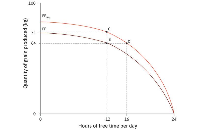
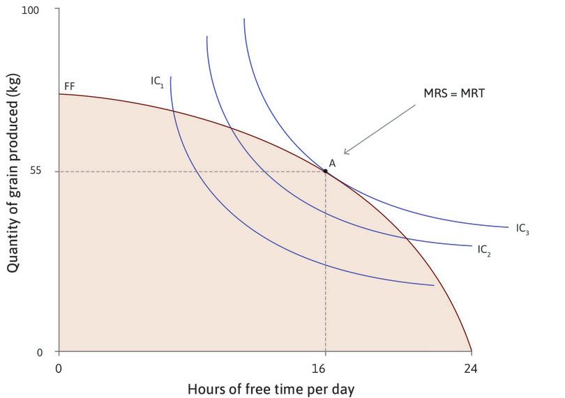
Figure 3.15 An improvement in technology expands Angela’s feasible set.
Now we add Angela’s indifference curves to the diagram, representing her preferences for free time and grain consumption, to find which combination in the feasible set is best for her. Figure 3.14 shows that her optimal choice under the original technology is to work for 8 hours a day, giving her 16 hours of free time and 55 units of grain. This is the point of tangency, where her two trade-offs balance out: her marginal rate of substitution (MRS) between grain and free time (the slope of the indifference curve) is equal to the MRT (the slope of the feasible frontier). We can think of the combination of free time and grain at point A as a measure of her standard of living.
Follow the steps in Figure 3.16 to see how her choice changes as a result of technological progress.
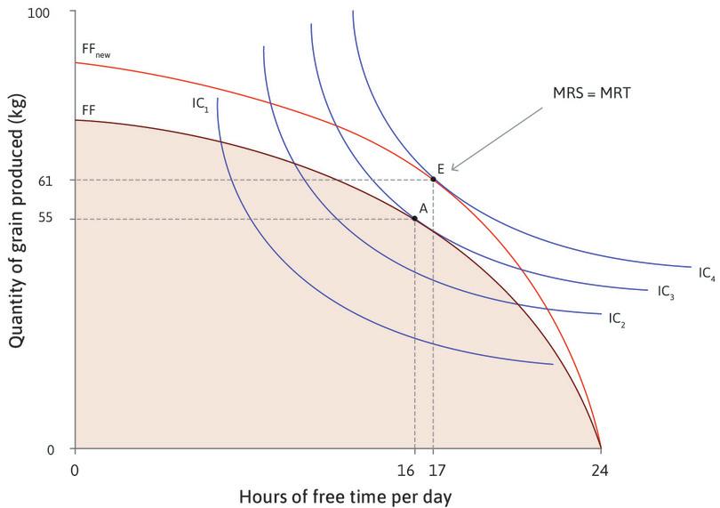
Figure 3.16 Angela’s choice between free time and grain.
Maximizing utility with the original technology
MRS = MRT for maximum utility
Technological progress
Angela’s new optimal choice
Technological change raises Angela’s standard of living: it enables her to achieve higher utility. Note that in Figure 3.16 she increases both her consumption of grain and her free time.
It is important to realize that this is just one possible result. Had we drawn the indifference curves or the frontier differently, the trade-offs Angela faces would have been different. We can say that the improvement in technology definitely makes it feasible to both consume more grain and have more free time, but whether Angela will choose to have more of both depends on her preferences between these two goods, and her willingness to substitute one for the other.
To understand why, remember that technological change makes the production function steeper: it increases Angela’s marginal product of labour. This means that the opportunity cost of free time is higher, giving her a greater incentive to work. But also, now that she can have more grain for each amount of free time, she may be more willing to give up some grain for more free time: that is, reduce her hours of work.
These two effects of technological progress work in opposite directions. In Figure 3.16, the second effect dominates and she chooses point E, with more free time as well as more grain. In the next section, we look more carefully at these two opposing effects, using a different example to disentangle them.
Question 3.9 Choose the correct answer(s)
The figures show Sakina’s production function and her corresponding feasible frontier for value of output/income and hours of work or free time per day. They show the effect of an improvement in her work technique, represented by the tilting up of the two curves.
Consider now two cases of further changes in Sakina’s environment:
Case A. She suddenly finds herself needing to spend 4 hours a day caring for a family member. (You may assume that her marginal product of labour is unaffected for the hours that she works.)
Case B. For health reasons her marginal product of labour for all hours is reduced by 10%.
Then:
- With Sakina’s marginal product of labour unaffected, the production function remains the same: each number of hours worked yields the same output as before.
- The feasible frontier shifts to the left and intersects the horizontal axis at 20 hours, since 4 hours a day are now spent on care, so any given number of hours committed to free time per day now corresponds to fewer hours worked and thus a lower output.
- With the reduction in Sakina’s marginal product of labour, the production function curve becomes flatter. This leads to tilting of the curve inwards, pivoted at the origin.
- The reduction in the marginal product results in a lower mark for every level of hours worked (except at zero), so the feasible frontier pivots around the intercept, rotating downwards.
Exercise 3.7 Sakina’s production function
We looked at the impact of a technological improvement in Angela’s feasible frontier. Now consider Sakina’s production function from Figure 3.7, and answer the following questions (we assume value of output is the same as income).
- What could bring about a technological improvement in Sakina’s production function?
- Draw a diagram to illustrate how this improvement would affect her feasible set of income and work hours.
- Analyse what might happen to her choice of work hours.
3.8 Income and substitution effects on hours of work and free time
Imagine that you are looking for a job after you leave college. You expect to be able to earn a wage of Rs. 15 per hour. Jobs differ according to the number of hours you have to work—so what would be your ideal number of hours? Together, the wage and the hours of work will determine how much free time you will have, and your total earnings.
We will work in terms of daily average free time and consumption, as we did for Angela. We will assume that your spending—that is, your average consumption of food, accommodation, and other goods and services—cannot exceed your earnings (for example, you cannot borrow to increase your consumption). If we write w for the wage, and you have t hours of free time per day, then you work for (24 − t) hours, and your maximum level of consumption, c, is given by:
\[c= w(24-t)\]- budget constraint
- An equation that represents all combinations of goods and services that one could acquire that exactly exhaust one’s budgetary resources.
We will call this your budget constraint, because it shows what you can afford to buy.
In the table in Figure 3.17 we have calculated your free time for hours of work varying between 0 and 16 hours per day, and your maximum consumption, when your wage is w = Rs. 15.
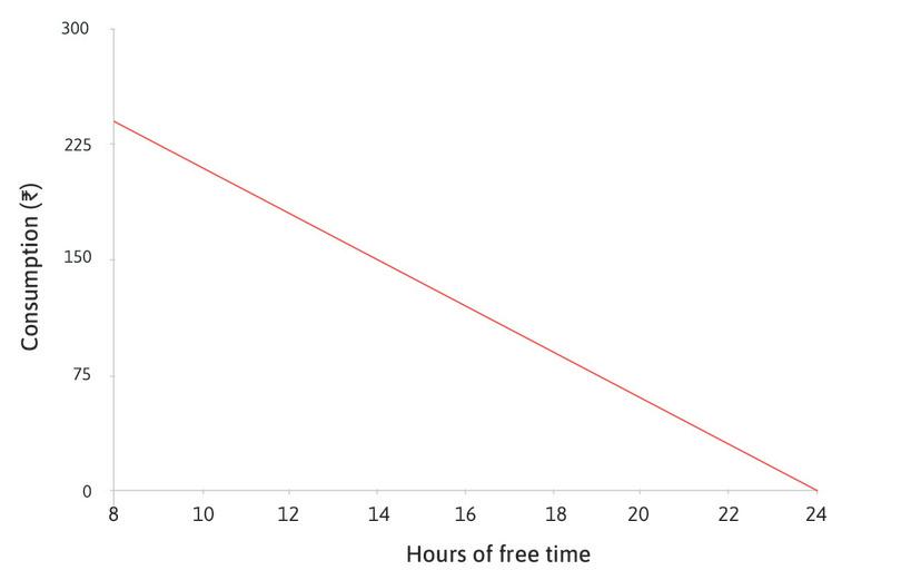
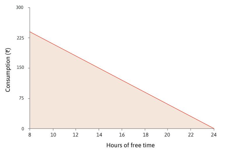
Figure 3.17 shows the two goods in this problem: hours of free time (t) on the horizontal axis, and consumption (c) on the vertical axis. When we plot the points shown in the table, we get a downward-sloping straight line: this is the graph of the budget constraint. The equation of the budget constraint is:
\[c= 15(24-t)\]The slope of the budget constraint corresponds to the wage: for each additional hour of free time, consumption must decrease by Rs. 15. The area under the budget constraint is your feasible set. Your problem is quite similar to Angela’s problem, except that your feasible frontier is a straight line. Remember that for Angela the slope of the feasible frontier is both the MRT (the rate at which free time could be transformed into grain) and the opportunity cost of an hour of free time (the grain foregone). These vary because Angela’s marginal product changes with her hours of work. For you, the marginal rate at which you can transform free time into consumption, and the opportunity cost of free time, is constant and is equal to your wage (in absolute value): it is Rs. 15 for your first hour of work, and still Rs. 15 for every hour after that.
What would be your ideal job? Your preferred choice of free time and consumption will be the combination on the feasible frontier that is on the highest possible indifference curve. Work through Figure 3.17 to find the optimal choice.
| Hours of work | 0 | 2 | 4 | 6 | 8 | 10 | 12 | 14 | 16 |
| Free time, t | 24 | 22 | 20 | 18 | 16 | 14 | 12 | 10 | 8 |
| Consumption, c | 0 | Rs. 30 | Rs. 60 | Rs. 90 | Rs. 120 | Rs. 150 | Rs. 180 | Rs. 210 | Rs. 240 |
The equation of the budget constraint is c = w(24 − t)
The wage is w = Rs. 15, so the budget constraint is c = 15(24 − t)
Figure 3.17 Your preferred choice of free time and consumption.

| Hours of work | 0 | 2 | 4 | 6 | 8 | 10 | 12 | 14 | 16 |
| Free time, t | 24 | 22 | 20 | 18 | 16 | 14 | 12 | 10 | 8 |
| Consumption, c | 0 | Rs. 30 | Rs. 60 | Rs. 90 | Rs. 120 | Rs. 150 | Rs. 180 | Rs. 210 | Rs. 240 |
The equation of the budget constraint is c = w(24 − t)
The wage is w = Rs. 15, so the budget constraint is c = 15(24 − t)
The budget constraint
| Hours of work | 0 | 2 | 4 | 6 | 8 | 10 | 12 | 14 | 16 |
| Free time, t | 24 | 22 | 20 | 18 | 16 | 14 | 12 | 10 | 8 |
| Consumption, c | 0 | Rs. 30 | Rs. 60 | Rs. 90 | Rs. 120 | Rs. 150 | Rs. 180 | Rs. 210 | Rs. 240 |
The equation of the budget constraint is c = w(24 − t)
The wage is w = Rs. 15, so the budget constraint is c = 15(24 − t)
The slope of the budget constraint
| Hours of work | 0 | 2 | 4 | 6 | 8 | 10 | 12 | 14 | 16 |
| Free time, t | 24 | 22 | 20 | 18 | 16 | 14 | 12 | 10 | 8 |
| Consumption, c | 0 | Rs. 30 | Rs. 60 | Rs. 90 | Rs. 120 | Rs. 150 | Rs. 180 | Rs. 210 | Rs. 240 |
The equation of the budget constraint is c = w(24 − t)
The wage is w = Rs. 15, so the budget constraint is c = 15(24 − t)
The feasible set
| Hours of work | 0 | 2 | 4 | 6 | 8 | 10 | 12 | 14 | 16 |
| Free time, t | 24 | 22 | 20 | 18 | 16 | 14 | 12 | 10 | 8 |
| Consumption, c | 0 | Rs. 30 | Rs. 60 | Rs. 90 | Rs. 120 | Rs. 150 | Rs. 180 | Rs. 210 | Rs. 240 |
The equation of the budget constraint is c = w(24 − t)
The wage is w = Rs. 15, so the budget constraint is c = 15(24 − t)
Your ideal job
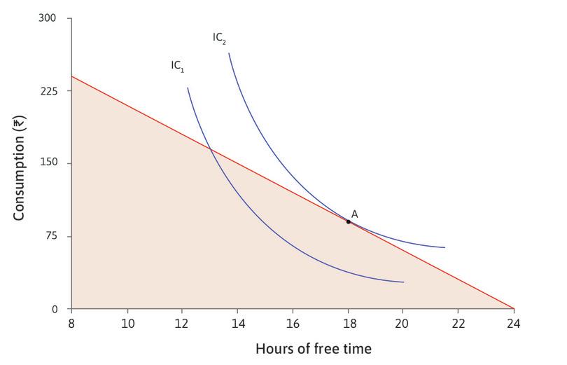
If your indifference curves look like the ones in Figure 3.17, then you would choose point A, with 18 hours of free time. At this point your MRS—the rate at which you are willing to swap consumption for time—is equal to the wage (Rs. 15, the opportunity cost of time). You would like to find a job in which you can work for 6 hours per day, and your daily earnings would be Rs. 90.
Like Sakina, you are balancing two trade-offs as shown in Figure 3.18.
| The trade-off | Where it is on the diagram | |
|---|---|---|
| MRS | Marginal rate of substitution: The amount of consumption you are willing to trade for an hour of free time. | The slope of the indifference curve. |
| MRT | Marginal rate of transformation: The amount of consumption you can gain from giving up an hour of free time, which is equal to the wage, w. | The slope of the budget constraint (the feasible frontier) which is equal to the wage. |
Figure 3.18 Your two trade-offs.
Your optimal combination of consumption and free time is the point on the budget constraint where:
\[\text{MRS = MRT} = w\]While considering this decision, you receive an email. A mysterious benefactor would like to give you an income of Rs. 50 a day—for life (all you have to do is provide your banking details.) You realize at once that this will affect your choice of job. The new situation is shown in Figure 3.19: for each level of free time, your total income (earnings plus the mystery gift) is Rs. 50 higher than before. So the budget constraint is shifted upwards by Rs. 50—the feasible set has expanded. Your budget constraint is now:
\[c = 15(24-t) + 50\]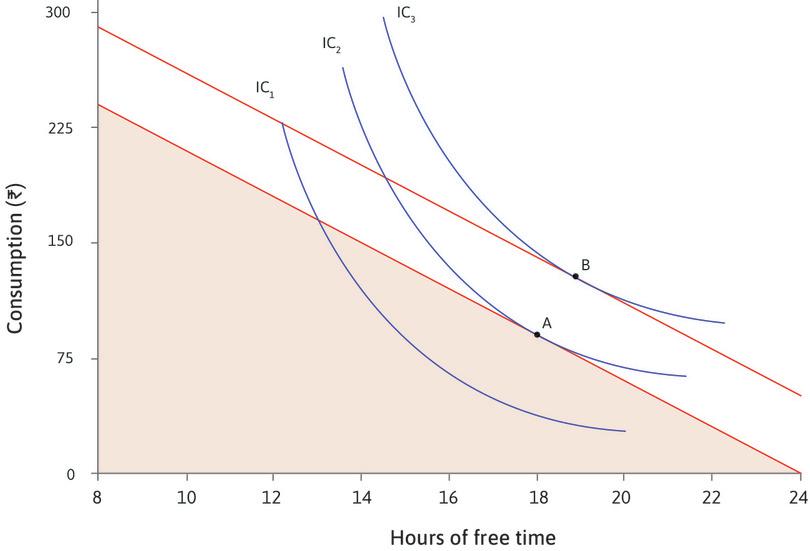
Figure 3.19 The effect of additional income on your choice of free time and consumption.
Notice that the extra income of Rs. 50 does not change your opportunity cost of time: each hour of free time still reduces your consumption by Rs. 15 (the wage). Your new ideal job is at B, with 19.5 hours of free time. B is the point on IC3 where the MRS is equal to Rs. 15. With the indifference curves shown in this diagram, your response to the extra income is not simply to spend Rs. 50 more; you increase consumption by less than Rs. 50, and you take some extra free time. Someone with different preferences might not choose to increase their free time: Figure 3.20 shows a case in which the MRS at each value of free time is the same on both IC2 and the higher indifference curve IC3. This person chooses to keep their free time the same, and consume Rs. 50 more.
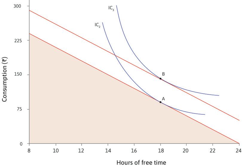
Figure 3.20 The effect of additional income for someone whose MRS doesn’t change when consumption rises.
- income effect
- The effect that the additional income would have if there were no change in the price or opportunity cost.
The effect of additional (unearned) income on the choice of free time is called the income effect. Your income effect, shown in Figure 3.19, is positive—extra income raises your choice of free time. For the person in Figure 3.20, the income effect is zero. We assume that for most goods the income effect will be either positive or zero, but not negative: if your income increased, you would not choose to have less of something that you valued.
You suddenly realize that it might not be wise to give the mysterious stranger your bank account details (perhaps it is a hoax). With regret you return to the original plan, and find a job requiring 6 hours of work per day. A year later, your fortunes improve: your employer offers you a pay rise of Rs. 10 per hour and the chance to renegotiate your hours. Now your budget constraint is:
\[c= 25(24-t)\]In Figure 3.21a you can see how the budget constraint changes when the wage rises. With 24 hours of free time (and no work), your consumption would be 0 whatever the wage. But for each hour of free time you give up, your consumption can now rise by Rs. 25 rather than Rs. 15. So your new budget constraint is a steeper straight line through (24, 0), with a slope equal to Rs. 25. Your feasible set has expanded. And now you achieve the highest possible utility at point D, with only 17 hours of free time. So you ask your employer if you can work longer hours—a 7-hour day.
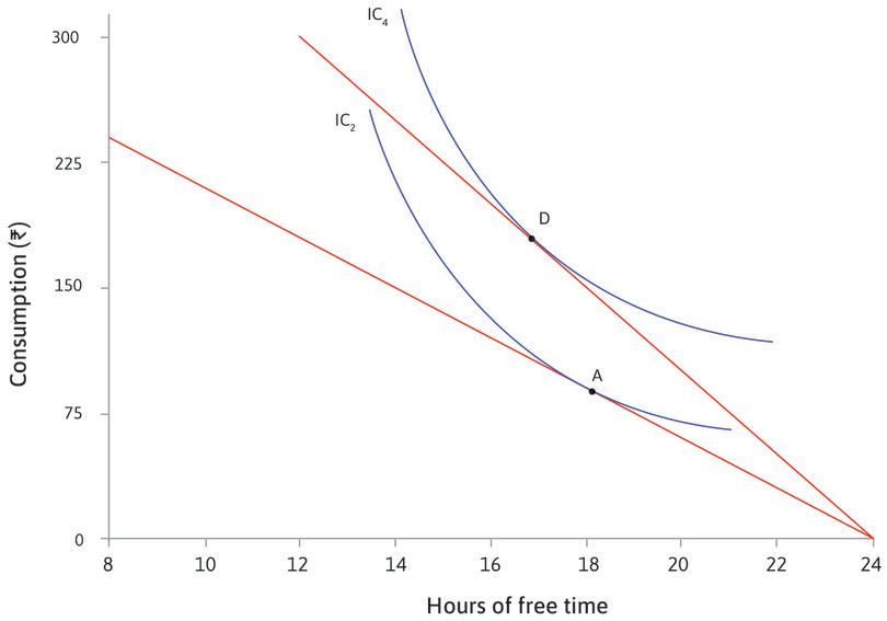
Figure 3.21a The effect of a wage rise on your choice of free time and consumption.
Compare the outcomes in Figure 3.20 and 3.21a. With an increase in unearned income you want to work fewer hours, while the wage increase in Figure 3.21a makes you decide to increase your working hours. Why does this happen? Because there are two effects of a wage increase:
- More income for every hour worked: For each level of free time you can have more consumption, and your MRS is higher: you are now more willing to sacrifice consumption for extra free time. This is the income effect we saw in Figure 3.19—you respond to additional income by taking more free time as well as increasing consumption.
- substitution effect
- The effect that is only due to changes in the price or opportunity cost, given the new level of utility.
- The budget constraint is steeper: The opportunity cost of free time is now higher. In other words, the marginal rate at which you can transform time into income (the MRT) has increased. And that means you have an incentive to work more—to decrease your free time. This is called the substitution effect.
Leibniz: Mathematics of income and substitution effects
The substitution effect captures the idea that when a good becomes more expensive relative to another good, you choose to substitute some of the other good for it. It is the effect that a change in the opportunity cost would have on its own, for a given utility level.
We can show both of these effects in the diagram. Before the wage rise you are at A on IC2. The higher wage enables you to reach point D on IC4. Figure 3.21b shows how we can decompose the change from A to D into two parts that correspond to these two effects.
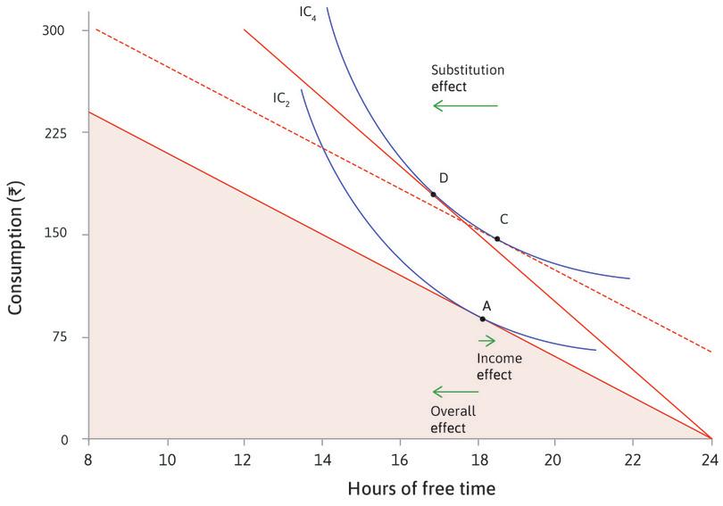
Figure 3.21b The effect of a wage rise on your choice of free time and consumption.
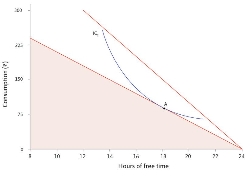
A rise in wages
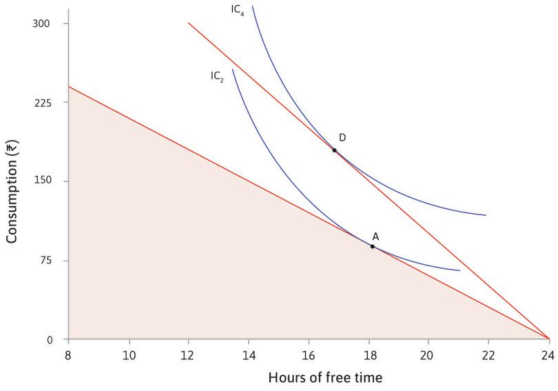
Now you can reach a higher indifference curve
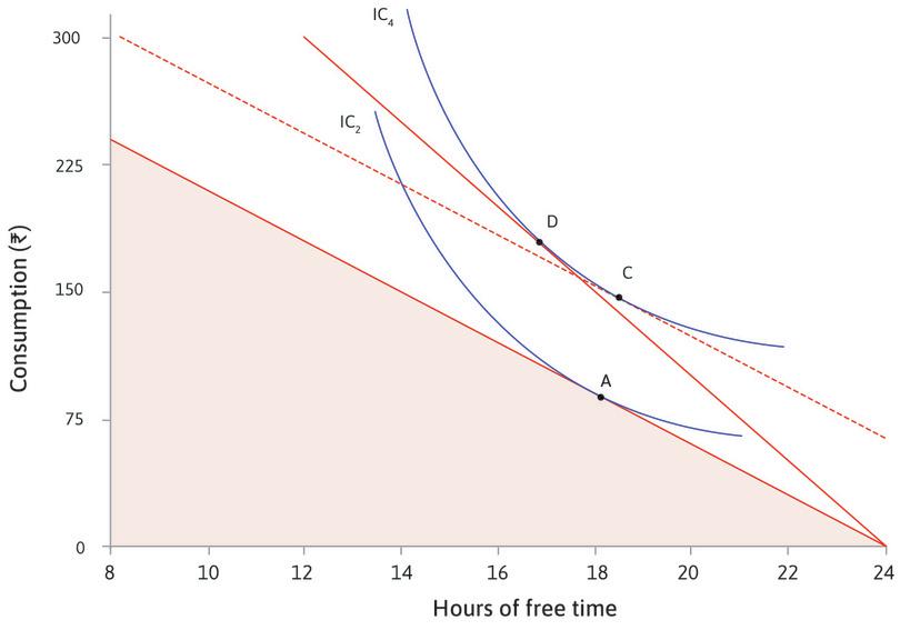
If there was no change in opportunity cost of free time
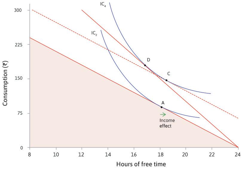
The income effect
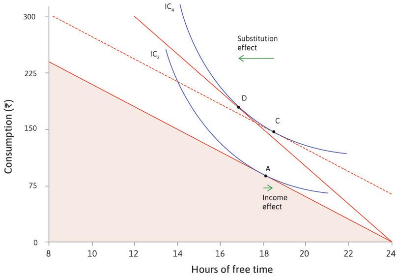
The substitution effect
The sum of the income and substitution effects
Income and substitution effects
A wage rise:
- raises your income for each level of free time, increasing the level of utility you can achieve
- increases the opportunity cost of free time
So it has two effects on your choice of free time:
- The income effect (because the budget constraint shifts outwards): the effect that the additional income would have if there were no change in the opportunity cost.
- The substitution effect (because the slope of the budget constraint, the MRT, rises): the effect of the change in the opportunity cost, given the new level of utility.
You can see in Figure 3.21b that with indifference curves of this typical shape a substitution effect will always be negative: with a higher opportunity cost of free time you choose a point on the indifference curve with a higher MRS, which is a point with less free time (and more consumption). The overall effect of a wage rise depends on the sum of the income and substitution effects. In Figure 3.21b the negative substitution effect is bigger than the positive income effect, so free time falls.
Technological progress
If you look back at Section 3.7, you will see that Angela’s response to a rise in productivity was also determined by these two opposing effects: an increased incentive to work produced by the rise in the opportunity cost of free time, and an increased desire for free time when her income rises.
We used the model of the self-sufficient farmer to see how technological change can affect working hours. Angela can respond directly to the increase in her productivity brought about by the introduction of a new technology. Employees also become more productive as a result of technological change, and if they have sufficient bargaining power, their wages will rise. The model in this section suggests that, if that happens, technological progress will also bring about a change in the amount of time employees wish to spend working.
The income effect of a higher wage makes workers want more free time, while the substitution effect provides an incentive to work longer hours. If the income effect dominates the substitution effect, workers will prefer fewer hours of work.
Question 3.10 Choose the correct answer(s)
Figure 3.21b depicts your budget constraint when the hourly wage is Rs. 15.
Which of the following is (are) true?
- For every additional hour of free time, you have Rs. 15 less to spend on consumption, so the slope of the budget constraint is −15.
- The budget constraint is the feasible frontier of the available combinations of free time and consumption. Its slope is constant, so the MRT is constant.
- An increase in the wage rate would make the budget constraint steeper, pivoted at the intercept on the horizontal axis, as every hour of free time would now cost more in foregone consumption.
- A gift would shift the budget constraint outward in a parallel manner, as the consumer could consume more at any given level of free time.
3.9 Is this a good model?
We have looked at two different contexts in which people decide how long to spend working—Sakina, a textile worker and Angela, a self-sufficient farmer. In each case we have modelled their preferences and feasible set, and the model tells us that their best (utility-maximizing) choice is the level of working hours at which the slope of the feasible frontier is equal to the slope of the indifference curve.
You may have been thinking: this is not what people do!
Billions of people organize their working lives without knowing anything about MRS and MRT (if they did make decisions that way, perhaps we would have to subtract the hours they would spend making calculations). And even if they did make their choice using mathematics, most of us can’t just leave work whenever we want. So how can this model be useful?
Remember from Unit 2 that models help us ‘see more by looking at less’. Lack of realism is an intentional feature of this model, not a shortcoming.
Trial and error replaces calculations
Can a model that ignores how we think possibly be a good model of how we choose?
Milton Friedman, an economist, explained that when economists use models in this way they do not claim that we actually think through these calculations (such as equating MRS to MRT) each time we make a decision. Instead we each try various choices (sometimes not even intentionally) and we tend to adopt habits, or rules of thumb that make us feel satisfied and not regret our decisions.
In his book Essays in positive economics, he described it as similar to playing billiards (pool):
Consider the problem of predicting the shots made by an expert billiard player. It seems not at all unreasonable that excellent predictions would be yielded by the hypothesis that the billiard player made his shots as if he knew the complicated mathematical formulas that would give the optimum directions of travel, could estimate accurately by eye the angles, etc., describing the location of the balls, could make lightning calculations from the formulas, and could then make the balls travel in the direction indicated by the formulas.
Our confidence in this hypothesis is not based on the belief that billiard players, even expert ones, can or do go through the process described. It derives rather from the belief that, unless in some way or other they were capable of reaching essentially the same result, they would not in fact be expert billiard players.3
Similarly, if we see a person not putting in much work on their farm, or asking for longer shifts after a pay rise, we do not need to suppose that this person has done the calculations we set out. If that person later regretted the choice, next time they might work harder on the farm, or cut their hours back. Eventually we could speculate they might end up with a decision on work time that is close to the result of our calculations.
That is why economic theory can help to explain, and sometimes even predict, what people do—even though those people are not performing the mathematical calculations that economists make in their models.
The influence of culture and politics
A second unrealistic aspect of the model: employers typically choose working hours, not individual workers, and employers often impose a longer working day than workers prefer. As a result, the hours that many people work are regulated by law, so that beyond some maximum amount neither the employee nor the employer can choose to work. In this case the government has limited the feasible set of hours and goods.
Although individual workers often have little freedom to choose their hours, it may nevertheless be the case that changes in working hours over time, and differences between countries, partly reflect the preferences of workers. If many individual workers in a democracy wish to lower their hours, they may ‘choose’ this indirectly as voters, if not individually as workers. Or they may bargain as members of a trade union for contracts requiring employers to pay higher overtime rates for longer hours.
This explanation stresses culture (meaning changes in preferences or differences in preferences among countries) and politics (meaning differences in laws, or trade union strength and objectives). They certainly help to explain differences in working hours between countries.
Cultures seem to differ. Some northern European cultures highly value their vacation times, while South Korea is famous for the long hours that employees put in. Legal limits on working time differ. In Belgium and France the normal work week is limited to 35–39 hours, while in Mexico the limit is 48 hours and in Kenya even longer.
But, even on an individual level, we may influence the hours we work. For example, employers who advertise jobs with the working hours that most people prefer may find they have more applicants than other employers offering too many (or too few) hours.
Remember, we also judge the quality of a model by whether it provides insight into something that we want to understand. In the next section, we will look at whether our model of the choice of hours of work can help us understand why working hours differ so much between countries and why, as we saw in the introduction, they have changed over time.
Exercise 3.8 Another definition of economics
Lionel Robbins, an economist, wrote in 1932 that: ‘Economics is the science that studies human behaviour as a relationship between given ends and scarce means which have alternative uses.’4
- Give an example from this unit to illustrate the way that economics studies human behaviour as a relationship between ‘given ends and scarce means with alternative uses’.
- Are the ‘ends’ of economic activity, that is, the things we desire, fixed? Use examples from this unit (working time and incomes, or working time and consumption) to illustrate your answer.
- The subject matter that Robbins refers to—doing the best you can in a given situation—is an essential part of economics. But is economics limited to the study of ‘scarce means which have alternative uses’? In answering this question, include a contrast between Robbins’ definition and the one given in Unit 1, and note that Robbins wrote this passage at a time when 15% of the British workforce was unemployed.
3.10 Explaining our working hours: Changes over time
During the year 1600, the average British worker was at work for 266 days. This statistic did not change much until the Industrial Revolution. Then, as we know from the previous unit, wages began to rise, and working time rose too: to 318 days in 1870.
Meanwhile, in the US, hours of work increased for many workers who shifted from farming to industrial jobs. In 1865 the US abolished slavery, and former slaves used their freedom to work much less. From the late nineteenth century until the middle of the twentieth century, working time in many countries gradually fell. Figure 3.1 at the beginning of this unit showed how annual working hours have fallen since 1870 in the Netherlands, the US and France.5
The simple models we have constructed cannot tell the whole story. Remember that the ceteris paribus assumption can omit important details: things that we have held constant in models may vary in real life.
As we explained in the previous section, our model omitted two important explanations, which we called culture and politics. Our model provides another explanation: economics.
Look at the two points in Figure 3.22, giving estimates of average amounts of daily free time and goods per day for employees in the US in 1900 and in 2013. The slopes of the budget constraints through points A and D are the real wage (goods per hour) in 1900 and in 2013. This shows us the feasible sets of free time and goods that would have made these points possible. Then we consider the indifference curves of workers that would have led workers to choose the hours they did. We cannot measure indifference curves directly: we must use our best guess of what the preferences of workers would have been, given the actions that they took.
How does our model explain how we got from point A to point D? You know from Figure 3.21b that the increase in wages would lead to both an income effect and a substitution effect. In this case, the income effect outweighs the substitution effect, so both free time and goods consumed per day go up. Figure 3.22 is thus simply an application to history of the model illustrated in Figure 3.21b. Work through the steps to see the income and substitution effects.
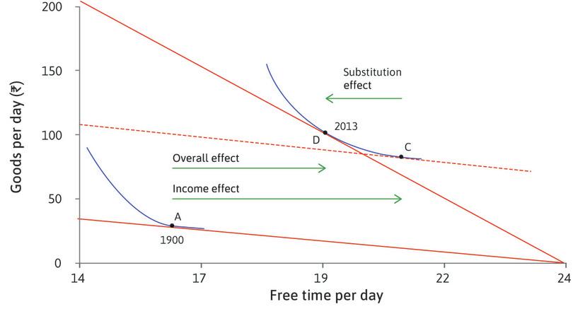
Figure 3.22 Applying the model to history: Increased goods and free time in the US (1900–2013).
OECD. Average annual hours actually worked per worker. Accessed June 2016. Michael Huberman and Chris Minns. 2007. ‘The times they are not changin’: Days and hours of work in Old and New Worlds, 1870–2000’. Explorations in Economic History 44 (4): pp. 538–567.
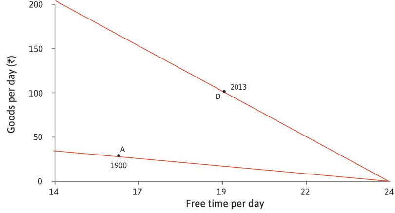
Using the model to explain historical change
OECD. Average annual hours actually worked per worker. Accessed June 2016. Michael Huberman and Chris Minns. 2007. ‘The times they are not changin’: Days and hours of work in Old and New Worlds, 1870–2000’. Explorations in Economic History 44 (4): pp. 538–567.
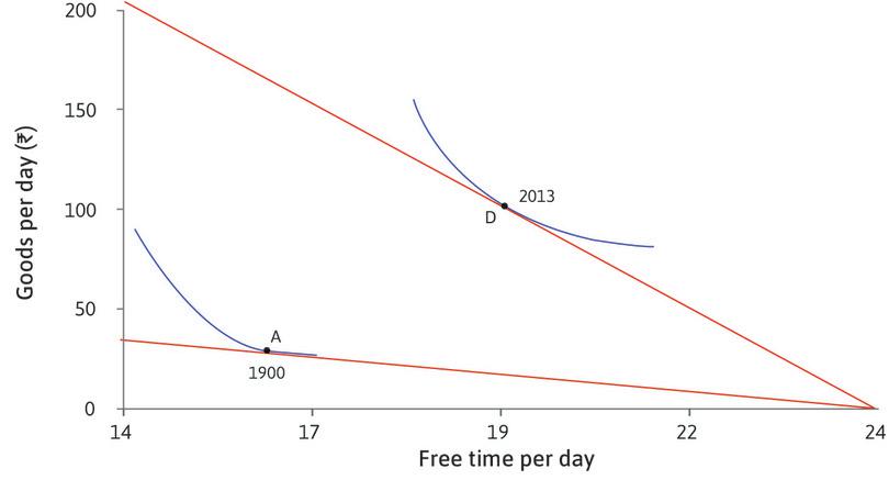
The indifference curves
OECD. Average annual hours actually worked per worker. Accessed June 2016. Michael Huberman and Chris Minns. 2007. ‘The times they are not changin’: Days and hours of work in Old and New Worlds, 1870–2000’. Explorations in Economic History 44 (4): pp. 538–567.
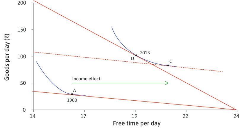
The income effect
OECD. Average annual hours actually worked per worker. Accessed June 2016. Michael Huberman and Chris Minns. 2007. ‘The times they are not changin’: Days and hours of work in Old and New Worlds, 1870–2000’. Explorations in Economic History 44 (4): pp. 538–567.
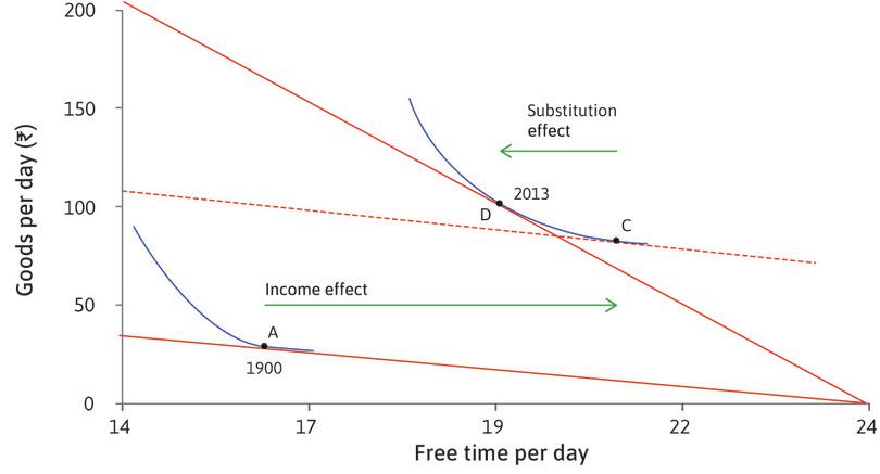
The substitution effect
OECD. Average annual hours actually worked per worker. Accessed June 2016. Michael Huberman and Chris Minns. 2007. ‘The times they are not changin’: Days and hours of work in Old and New Worlds, 1870–2000’. Explorations in Economic History 44 (4): pp. 538–567.
Income and substitution effects
OECD. Average annual hours actually worked per worker. Accessed June 2016. Michael Huberman and Chris Minns. 2007. ‘The times they are not changin’: Days and hours of work in Old and New Worlds, 1870–2000’. Explorations in Economic History 44 (4): pp. 538–567.
How could reasoning in this way explain the other historical data that we have?
First, consider the period before 1870 in Britain, when both working hours and wages rose:
- Income effect: At the relatively low level of consumption in the period before 1870, workers’ willingness to substitute free time for goods did not increase much when rising wages made higher consumption possible.
- Substitution effect: But they were more productive and paid more, so each hour of work brought more rewards than before in the form of goods, increasing the incentive to work longer hours.
- Substitution effect dominated: Therefore before 1870 the negative substitution effect (free time falls) was bigger than the positive income effect (free time rises), so work hours rose.
During the twentieth century we saw rising wages and falling working hours. Our model accounts for this change as follows:
- Income effect: By the late nineteenth century workers had a higher level of consumption and valued free time relatively more—their marginal rate of substitution was higher—so the income effect of a wage rise was larger.
- Substitution effect: This was consistent with the period before 1870.
- Income effect now dominates: When the income effect began to outweigh the substitution effect, working time fell.
We should also consider the possibility that preferences change over time. If you look carefully at Figure 3.1 you can see that in the last part of the twentieth century hours of work rose in the US, even though wages hardly increased. Hours of work also rose in Sweden during this period.
The term ‘conspicuous consumption’ was coined by Thorstein Veblen (1857–1929), an economist, in his book Theory of the Leisure Class. At the time, he was describing the habits only of the upper classes. But increasing disposable income during the twentieth century means the term is now applied to anyone who ostentatiously consumes expensive goods and services as a public display of wealth.
Thorstein Veblen. (1899) 2007. Theory of the Leisure Class. Oxford: Oxford University Press.
- conspicuous consumption
- The purchase of goods or services to publicly display one’s social and economic status.
Why? Perhaps Swedes and Americans came to value consumption more over these years. In other words, their preferences changed so that their MRS fell (they became more like today’s South Korean workers). This may have occurred because in both the US and Sweden the share of income gained by the very rich increased considerably, and the lavish consumption habits of the rich set a higher standard for everyone else. As a result, many people of lesser means tried to mimic the consumption habits of the rich, a habit known as conspicuous consumption. According to this explanation, Swedes and Americans were ‘keeping up with the Joneses’. The Joneses got richer, leading everyone else to change their preferences.
The combined political, cultural and economic influences on our choices may produce some surprising trends. In our ‘Economist in action’ video, Juliet Schor, a sociologist and economist who has written about the paradox that many of the world’s wealthiest people are working more despite gains in technology, asks what this means for our quality of life, and for the environment.

Question 3.11 Choose the correct answer(s)
Figure 3.22 depicts a model of labour supply and consumption for the US in 1900 and 2013. The wage rate is shown to have increased between the two years.
Which of the following are true?
- The substitution effect is the pure effect of the change in the slope of the budget constraint. The movement from A to D is the combined effect of the substitution and income effects.
- The income effect is the effect of a higher income on the choice of free time, which is shown by the parallel shift outwards of the budget constraint, and thus a move from A to C.
- With the indifference curves shown, the income effect of the wage increase is greater than the substitution effect, so overall free time increases and hours of work fall.
- With different indifference curves, the substitution effect could have dominated the income effect, leading to a reduction of free time between 1900 and 2013.
What about the future? The high-income economies will continue to experience a major transformation: the declining role of work in the course of our lifetimes. We go to work at a later age, stop working at an earlier age of our longer lives, and spend fewer hours at work during our working years. Robert Fogel, an economic historian, estimated the total working time, including travel to and from work and housework, in the past. He made projections for the year 2040, defining what he called discretionary time as 24 hours a day minus the amount we all need for biological maintenance (sleeping, eating and personal hygiene). Fogel calculated leisure time as discretionary time minus working time.6
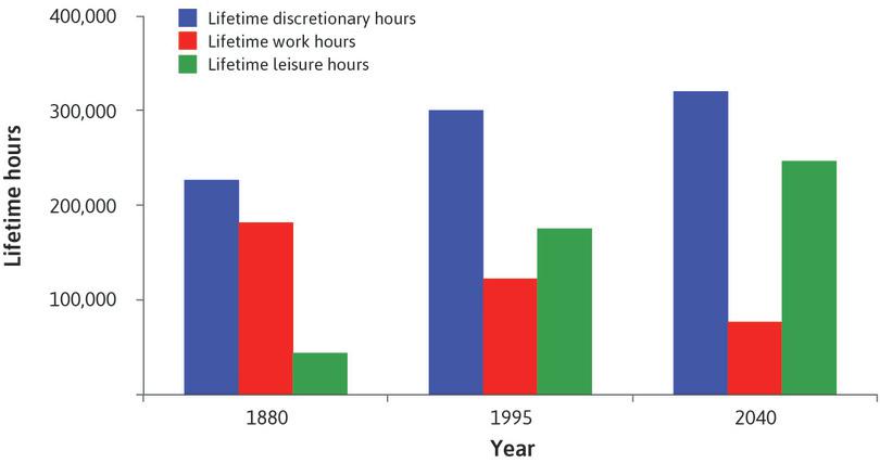
Figure 3.23 Estimated lifetime hours of work and leisure (1880, 1995, 2040).
Robert William Fogel. 2000. The Fourth Great Awakening and the Future of Egalitarianism. Chicago: University of Chicago Press.
In 1880 he estimated that lifetime leisure time was just a quarter of lifetime work hours. In 1995 leisure time exceeded working time over a person’s entire life. He predicted that lifetime leisure would be three times of lifetime working hours by the year 2040. His estimates are in Figure 3.23.
We do not yet know if Fogel has overstated the future decline in working time, as Keynes once did. But he certainly is right that one of the great changes brought about by the technological revolution is the vastly reduced role of work in the life of an average person.
Exercise 3.9 Scarcity and choice
- Do our models of scarcity and choice provide a plausible explanation for the observed trends in working hours during the twentieth century?
- What other factors, not included in the model, might be important in explaining what has happened?
- Remember Keynes’ prediction that working hours would fall to 15 hours per week in the century after 1930. Why do you think working hours have not changed as he expected? Have people’s preferences changed? The model focuses on the number of hours workers would choose, so do you think that many employees are now working longer than they would like?
- In his essay, Keynes said that people have two types of economic needs or wants: absolute needs that do not depend on the situation of other fellow humans, and relative needs—which he called ‘the desire for superiority’. The phrase ‘keeping up with the Joneses’ captures a similar idea that our preferences could be affected by observing the consumption of others. Could relative needs help to explain why Keynes was so wrong about working hours?
3.11 Explaining Women’s Labour Force Participation
‘Sakina’ is a real person (although the models describing her behaviour and name are made up). Economist Amit Basole studied the way women spent their time in Varanasi in 2006. Much as our model predicts, they described their decisions about how to spend their time working versus doing other things as a trade-off. A respondent in Basole’s field study explained, for example that ‘Whatever time I get after cooking three meals, I spend on this [Textile Production]’.7
Our model allows us to ask several questions. What might happen if the respondent’s partners had taken up some of the burden of cooking meals? What might happen to her choice of working? Similarly, what might happen if technological advances such as microwave ovens or washing machines lessened the time involved in unpaid labour (cooking, cleaning, and taking care of the children)? It should be clear that for the Sakina of our model, this would be equivalent to reducing the opportunity cost of paid working time since the unpaid labour that she normally does would take less time.
Depending on which effect dominated, the income effect or the substitution effect, Sakina would either spend more time in paid work or in taking actual leisure. This model can help us understand long-term trends like the ones we saw in Figure 3.3. To recall, Figure 3.3 shows that the female labour force participation in five high-income economies rose substantially since 1900. We can explain at least some of this increase by the fact that the ‘traditional’ areas in which women spent their time, unpaid home labour, became easier with the advent of domestic consumer goods such as vacuum cleaners and washing machines, freeing up time for paid work. Of course, this is not all that mattered. Certainly cultural and political patterns as well as the nature of work changed over the twentieth century and made it far more acceptable and possible for women to enter the labour force and for men to do unpaid caring labour.
In several countries such as India, as Figure 3.4 shows, however, that women still spend far more time on the latter than the former. Still, our model might predict that with technological changes that free up time from unpaid home labour, women may begin to participate in far greater numbers than before. What is equally possible is that as incomes go up, women and men who were working long hours, may choose to work less, or even to stop working (say, if a partner is making enough money for both of them) and withdraw from the labour force altogether.
Consider Sakina’s family. It consists of her, her husband Arif, and two children. Sakina and Arif make their decisions on work jointly, trying to take into account what they need every month. If his income is insufficient to make ends meet, Sakina works to make up the difference. For the sake of simplicity, let us assume that both Arif and Sakina earn the same amount per hour of work. What happens then if wages rise in the textile industry?
At this point they face a choice. If, as a family, the income effect of wage increases dominates the substitution effect, they will choose to work less hours. In our story, it is possible that Sakina does not have to work at all now to make up the difference. So, if for a family the income effect dominated the substitution effect, one might even see women cutting their hours of work to zero and leaving the paid labour force.
Figure 3.24 shows what has been happening to women’s labour force participation in India since 2004. As can be seen, women in the middle age ranges are more likely to be part of the labour force than younger or older women. Interestingly, the figure shows that women are less likely to be part of the labour force now than in 2011. There could be many reasons to explain this: for example, it has become harder for women to get jobs that are desirable. But it could also be explained by our model. If families decide that they have enough money jointly or if one person, say the husband, is earning more as income rises, they may agree that the wife does not need to undertake paid work. So, if for a family the income effect dominated the substitution effect, one might see this pattern.
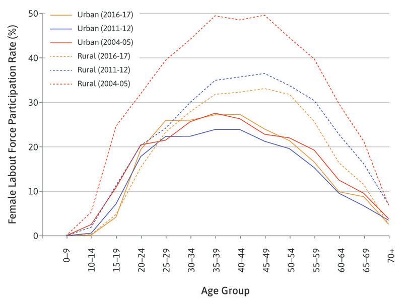
Figure 3.24 Female Labour Force Participation in India, by age group (2004, 2011, 2016).
NSS-EUS Surveys 2004, 2011. PLFS 2016-17
Exercise 3.10 Technological Change and free time
Hans Rosling describes, in this video, the impact that the advent of the washing machine had on the time available to his grandmother.
What other kinds of technology have these effects? How do you think the work at home should be apportioned?

3.12 Conclusion
We have used a model of decision making under scarcity to analyse choices of hours of work. This was used to understand why working hours have fallen over the last century as well as the possible reasons as to why women and men work differently. People’s preferences with respect to goods and free time are described by indifference curves, and their production function (or budget constraint) determines their feasible set. The choice that maximizes utility is a point on the feasible frontier where the marginal rate of substitution (MRS) between goods and free time is equal to the marginal rate of transformation (MRT).
An increase in productivity or wages alters the MRT, raising the opportunity cost of free time. This provides an incentive to work longer hours (the substitution effect). But higher income may increase the desire for free time (the income effect). The overall change in hours of work depends on which of these effects is bigger.
Concepts introduced in Unit 3
Before you move on, review these definitions:
3.13 References
- Basole, Amit. 2016. ‘Spare Change for Spare Time? Homeworking Women in Banaras’. Women Workers in Urban India. Cambridge: Cambridge University Press.
- Carmichael, Fiona, Claire Hulme, Sally Sheppard, and Gemma Connell. 2008. ‘Work – life imbalance: Informal care and paid employment in the UK’. Feminist Economics 14 (2): pp. 3–35.
- Fogel, Robert William. 2000. The Fourth Great Awakening and the Future of Egalitarianism. Chicago: University of Chicago Press.
- Harford, Tim. 2015. ‘The rewards for working hard are too big for Keynes’s vision’. The Undercover Economist. First published by The Financial Times. Updated 3 August 2015.
- Keynes, John Maynard. 1963. ‘Economic Possibilities for our Grandchildren’. In Essays in Persuasion, New York, NY: W. W. Norton & Co.
- Plant, E. Ashby, K. Anders Ericsson, Len Hill, and Kia Asberg. 2005. ‘Why study time does not predict grade point average across college students: Implications of deliberate practice for academic performance’. Contemporary Educational Psychology 30 (1): pp. 96–116.
- Robbins, Lionel. 1984. An Essay on the Nature and Significance of Economic Science. New York: New York University Press.
- Schor, Juliet B. 1992. The Overworked American: The Unexpected Decline Of Leisure. New York, NY: Basic Books.
- Veblen, Thorstein. 2007. The Theory of the Leisure Class. Oxford: Oxford University Press.
- Whaples, Robert. 2001. ‘Hours of work in U.S. History’. EH.Net Encyclopedia.
-
John Maynard Keynes. 1963. ‘Economic Possibilities for our Grandchildren’. In Essays in Persuasion, New York, NY: W. W. Norton & Co. ↩
-
Tim Harford. 2015. ‘The rewards for working hard are too big for Keynes’s vision’. The Undercover Economist. First published by The Financial Times. Updated 3 August 2015. ↩
-
Milton Friedman. 1953. Essays in positive economics, 7th ed. Chicago: University of Chicago Press. ↩
-
Lionel Robbins. 1984. An essay on the nature and significance of economic science, 3rd ed. New York: New York University Press. ↩
-
Robert Whaples. 2001. ‘Hours of work in U.S. History’ EH.Net Encyclopedia. ↩
-
Robert William Fogel. 2000. The fourth great awakening and the future of egalitarianism: The political realignment of the 1990s and the fate of egalitarianism. Chicago: University of Chicago Press. ↩
-
Amit Basole. 2016. ‘Spare Change for Spare Time? Homeworking Women in Banaras’. Women Workers in Urban India. Cambridge University Press. ↩
