Leibniz
3.4.1 Marginal rate of transformation
Sakina’s decision of how much to work is constrained by the feasible set of combinations of free time and income. So she faces a trade-off: to get a good income via cloth production, she has to give up some free time. The marginal rate of transformation (MRT) measures the size of the trade-off. Here we show how the MRT can be calculated from the production function.
The equation of the feasible frontier
Figure 1 shows Sakina’s feasible set. Recall that we constructed the feasible frontier using a production function that relates value of output (income) to hours of work.
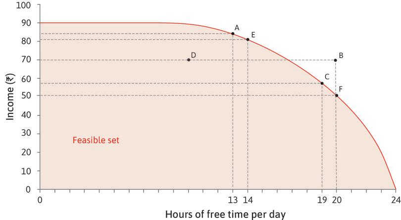
Figure 1 How does Sakina’s choice of free time affect her income?
To see this mathematically, let Sakina’s production function be (as before):
\[y = f(h)\]where \(y\) is her value of output (her income) and \(h\) her hours of work, and \(f\) is an increasing function.
The feasible frontier is the relationship between her free time and income. If Sakina takes \(t\) hours of free time, her hours of work are:
\[h=24-t\]Substituting this into the production function, we obtain the equation of the feasible frontier:
\[y = f(24 - t)\]Calculating the marginal rate of transformation
We have seen diagrammatically that the MRT is related to the slope of the feasible frontier. We can find the slope by differentiating the equation of the feasible frontier. When Sakina has \(t\) hours of free time, the rate at which her income changes as free time increases is given by:
\[\frac{dy}{dt} = f'(24-t)\frac{d}{dt}(24 -t)\]using the composite function rule (sometimes called the chain rule). Simplifying,
\[\frac{dy}{dt} = - f'(24-t)\]The right-hand side of this equation is negative, since \(f\) is an increasing function. Thus, the frontier slopes downward, as in the diagram. The slope of the feasible frontier at the point \((t,\ f(24 -t))\) is the negative quantity \(-f'(24 -t)\).
- marginal rate of transformation (MRT)
- The quantity of some good that must be sacrificed to acquire one additional unit of another good. At any point, it is the slope of the feasible frontier. See also: marginal rate of substitution.
The negative slope tells us that the income decreases as free time increases. The marginal rate of transformation (MRT) is the rate at which the income increases as free time is given up, which is given by the absolute value of the slope, a positive quantity:
\[\text{MRT}=f'(24-t)\]The meaning of the MRT is as follows: if free time increases by a small amount, say \(\Delta t\) hours, income decreases by approximately \(f'(24-t)\Delta t\) rupees. Or if free time decreases by \(\Delta t\) hours, income increases by approximately \(f'(24-t)\Delta t\) rupees. Figure 2 shows the feasible frontier for the production function \(y=28h^{1.6}\) (which has a similar, but not identical, shape to Sakina’s feasible frontier). The lower panel shows the MRT, which rises as we move to the right along the frontier, increasing free time and lowering income.
To summarize, the MRT measures the rate at which income has to be given up if hours of free time increase, and can be found by simply differentiating the production function. Since the number of hours of work \(h\) is equal to \(24 - t\), the MRT is the same as the marginal product of labour \(f'(h)\). The fact that the MRT rises as we move along the frontier in the direction of more free time and fewer hours of work is a consequence of diminishing returns to labour: since \(f'(h)\) is a decreasing function of \(h\), it rises when \(h\) falls.
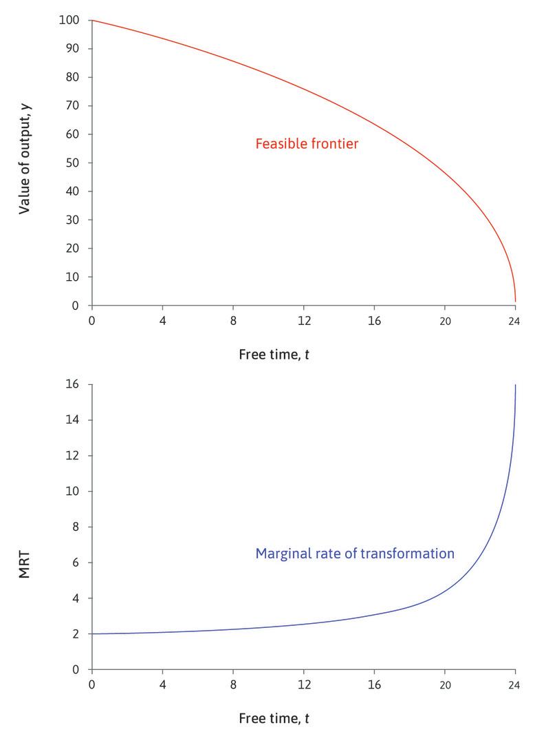
Figure 2 The feasible frontier \(y = 28(24-t)^{1.6}\), and the corresponding marginal rate of transformation.
