Unit 7 The firm and its customers
How a profit-maximizing firm producing a differentiated product interacts with its customers
- Firms producing differentiated products choose price and quantity to maximize their profits, taking into account the product demand curve and the cost function.
- The responsiveness of consumers to a price change is measured by the elasticity of demand, which affects the firm’s price and profit margin.
- When consumers and firm owners interact in markets, the gains from trade are shared, but when prices are set above marginal cost there is market failure and deadweight loss.
- Economic policymakers use estimates of elasticities of demand to design tax policies, and reduce firms’ market power through competition policy.
In the late 1990s the terrible spectre of AIDS was haunting sub-Saharan Africa. By the year 2000, one in every four pregnant women were HIV positive.1
At the time, demographers expected about five million people to die in the next decade as a result of the disease.2 This catastrophic human disaster was also expected to become worse, with the number of deaths increasing. This was largely because the only treatment course at that point was prohibitively expensive. The medicine at that time, a triple combination of antiretrovirals (ARVs), was being offered by a group of multinational pharmaceutical companies. The lowest cost offered to a limited set of countries was about $1,000 per year—well beyond the capacity of almost everyone in the affected region. In more developed countries, the price could go up to $15,000 a year.
But things were about to change. In early 2001, an Indian pharmaceutical company, Cipla, offered the same triple-combination of ARVs for $350 per patient per year (or less than one dollar per day). Moreover, they officially announced this lower price to all countries. This dramatic price reduction received huge media attention, and the multinational companies reduced their prices sharply too. Figure 7.1 shows the fall in per person cost of various ARVs per year during the period 2000 to 2011. In the years that followed, treatment finally become affordable to the majority of the population and several million lives were potentially saved or improved.3
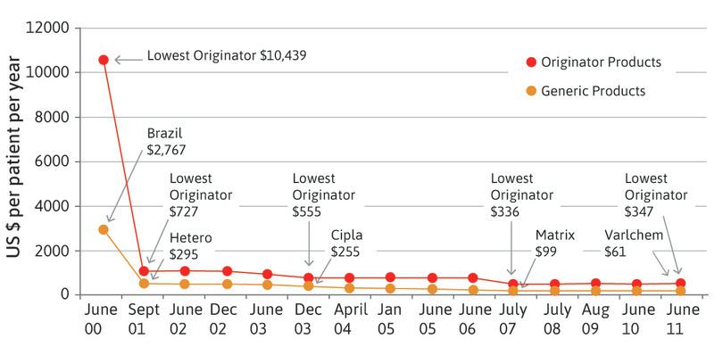
Figure 7.1 Per person cost of ARV courses per year (in US $).
Graph 3 in ‘Untangling the web of antiretroviral price reductions’. Médecins Sans Frontières. July 2011.
How and why did the multinational drug companies decide to price the drugs the way they did before 2001 and after the announcement by Cipla? How did Cipla choose its price? More generally, how do firms decide to undertake production decisions and pricing decisions when they face more or less competition? Why are some firms more successful than others? And why do some firms grow while others remain small or go out of business?
Firms have many decisions to make. For example, how to choose, design, and advertise products that will attract customers; how to produce at lower cost and at a higher quality than their competitors; or how to recruit and retain employees who can make these things happen. In this unit, we look at one of the most important of these decisions: how to choose the price and quantity to produce. This depends on demand, that is, the willingness of potential consumers to pay for the product, and production costs. We also look at markets, in which the decisions of firms and consumers come together to determine the allocation of goods and services.
How did Cipla decide its pricing strategy? Keeping the price low, as Cipla did, is one possible strategy for a firm seeking to maximize its profits. Even though the profit on each item is small, the low price may attract so many customers that total profit is high. On the other hand, charging a higher price may also be a viable strategy. Even if they sold a small number of units, the profit on each unit may be large. The first firm to do this was GlaxoSmithKline, another pharmaceutical company.
Figure 7.2 illustrates key decisions that a firm makes.
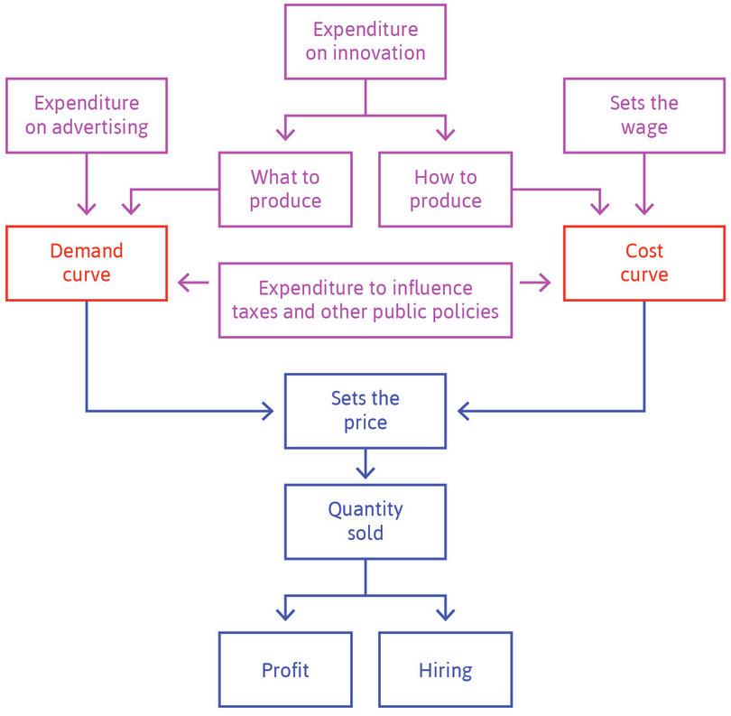
Figure 7.2 Decision-making process of a firm.
7.1 Economies of scale and the cost advantages of large-scale production
Many of the firms we have spoken about are fairly large. For example, Both Cipla and GlaxoSmithKline have about 23,000 and 100,000 employees respectively. Many of the other firms that we know of are also very large. Think about companies like Intel, FedEx, Walmart, and others. But some other firms, especially some of those discussed in Unit 6, are not. Why is this the case? An important reason why a large firm may be more profitable than a small firm is that the large firm produces its output at lower cost per unit. This may be possible for two reasons:
- Technological advantages: Large-scale production often uses fewer inputs per unit of output.
- Cost advantages: In larger firms, costs that don’t depend on number of units produced (such as advertising or acquiring the necessary patents or other intellectual property rights (IPR)), have a smaller effect on the cost per unit.
Technological advantages
- economies of scale
- These occur when doubling all of the inputs to a production process more than doubles the output. The shape of a firm’s long-run average cost curve depends both on returns to scale in production and the effect of scale on the prices it pays for its inputs. Also known as: increasing returns to scale. See also: diseconomies of scale.
- increasing returns to scale
- These occur when doubling all of the inputs to a production process more than doubles the output. The shape of a firm’s long-run average cost curve depends both on returns to scale in production and the effect of scale on the prices it pays for its inputs. Also known as: economies of scale. See also: decreasing returns to scale, constant returns to scale.
Economists use the term economies of scale or increasing returns to describe the technological advantages of large-scale production. For example, if doubling the amount of every input that the firm uses triples the firm’s output, then the firm exhibits increasing returns.
Economies of scale may result from specialization within the firm, which allows employees to do the task they do best and minimizes training time by limiting the skill set that each worker needs. Economies of scale may also occur for purely engineering reasons. For example, transporting more of a liquid requires a larger pipe, but doubling the capacity of the pipe increases its diameter (and the material necessary to construct it) by much less than a factor of two.
Cost advantages
- fixed costs
- Costs of production that do not vary with the number of units produced.
- research and development
- Expenditures by a private or public entity to create new methods of production, products, or other economically relevant new knowledge.
There is usually a fixed cost of production to a firm. It does not depend on the number of units, and so would be the same whether the firm produced one unit or many. Examples of fixed costs include:
- Marketing expenses: For example, advertising. The cost of running a 10-second advertisement during the India-Pakistan World Cup match in 2019 was Rs. 25 lakh per 10 seconds, which would be justifiable only if a large number of units would be sold as a result.
- Innovation: For example, research and development (R&D), product design, acquiring a production licence, or obtaining a patent for a particular technique.
- Lobbying: The cost of trying to influence government bodies, or of contributions to election campaigns and public relations expenditures, are more or less independent of the level of the firm’s output.
Demand advantages
- network economies of scale
- These exist when an increase in the number of users of an output of a firm implies an increase in the value of the output to each of them, because they are connected to each other.
Large size can also benefit a firm in selling its product, if people are more likely to buy a product or service that already has a lot of users. For example, a software application is more useful when everybody else uses a compatible version. These demand-side benefits of scale are called network economies of scale. There are many examples in technology-related markets.
Organizational disadvantages
- diseconomies of scale
- These occur when doubling all of the inputs to a production process less than doubles the output. Also known as: decreasing returns to scale. See also: economies of scale.
Production by a small group of people is therefore often too costly to compete with larger firms. But while small firms typically either grow or die, there are limits to growth known as diseconomies of scale, or decreasing returns.
A larger firm needs more layers of management and supervision. Firms typically organize themselves as hierarchies in which employees are supervised by those at a higher level and, as the firm grows, the organizational costs will grow as a proportion of the firm’s overall costs.
Outsourcing
Sometimes it is cheaper to outsource production of part of the product than to manufacture it within the firm. For example, Apple would be even more gigantic if its employees produced the touchscreens, chipsets, and other components that make up the iPhone and iPad, rather than purchasing these parts from Toshiba, Samsung, and other suppliers. Apple’s outsourcing strategy limits the firm’s size and increases the size of Toshiba, Samsung, and other firms that produce Apple’s components. In our ‘Economist in action’ video Richard Freeman, an economist who specializes in labour markets, explains some of the consequences of outsourcing.

Question 7.1 Choose the correct answer(s)
Which of the following are factors that contribute to a firm’s diseconomies of scale?
- Doubling of the capacity of a pipe requires less than doubling of the material required to construct it. This leads to economies of scale.
- Fixed costs per unit of output decrease as the level of output increases. This leads to economies of scale.
- If you only have one employee, then you can make sure that he works hard. You cannot do this when there are 100 workers. This leads to diseconomies of scale.
- The network effect occurs when people are more likely to buy the firm’s product or service if there are already a lot of users (for example, word processing software). This contributes to the firm’s economies of scale.
7.2 The demand curve and willingness to pay
The demand for a product will depend on its price, and the costs of production may depend on how many units are produced. But a firm can actively influence both consumer demand and costs in more ways than through price and quantity. As we saw in Unit 2, innovation may lead to new and attractive products, or to lower production costs. If the firm can innovate successfully it can earn economic rents—at least in the short term until others catch up. Further innovation may be needed if it is to stay ahead. Advertising can increase demand. And as we saw in Unit 6, the firm sets the wage, which is an important component of its cost. As we will see in later units, the firm also spends to influence taxes and environmental regulation in order to lower its production costs.
The demand curve and differentiated products
- demand curve
- The curve that gives the quantity consumers will buy at each possible price.
To decide what price to charge and how much to produce, a firm needs information about demand: how much potential consumers are willing to pay for its product. This information is summarized in a demand curve.
In 1996, Jerry Hausman, an economist, used data on weekly sales of family breakfast cereals in US cities to estimate how the weekly quantity of cereal that customers in a typical city would wish to buy would vary with its price per pound (there are 2.2 pounds in 1 kg). For example, you can see from Figure 7.3 that if the price were $3, customers would demand 25,000 pounds of Apple-Cinnamon Cheerios. For most products, the lower the price, the more customers wish to buy.
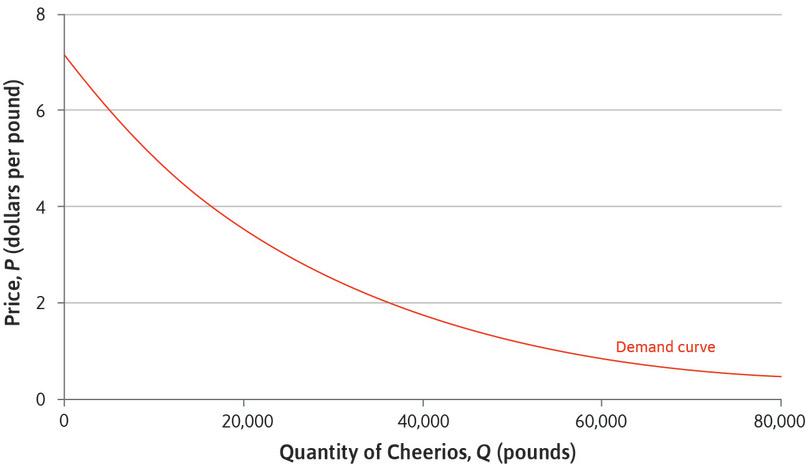
Figure 7.3 Estimated demand for Apple-Cinnamon Cheerios
Breakfast cereals are differentiated products. Each brand is produced by just one firm and has some unique nutritional, taste, and other characteristics that distinguish it from the brands sold by other firms.
Many other consumer goods and services are also differentiated products. If you want to buy a car, a mobile phone, or a washing machine, it is not just the price that matters—you will want to find a brand and model with characteristics that match your own preferences. You might consider the design, the quality, or the service the manufacturer offers, rather than always choosing the cheapest.
What this means is that even if there are many firms selling similar products, each firm is alone as a seller of its particular type and brand. Only one firm sells Apple Cinnamon Cheerios: General Mills.
How economists learn from facts Estimating demand curves using surveys
Jerry Hausman used data on cereal purchases to estimate the demand curve for Apple-Cinnamon Cheerios. Another method, particularly useful for firms introducing completely new products, is a consumer survey. Suppose you were investigating the potential demand for space tourism. You could try asking potential consumers:
‘How much would you be willing to pay for a 10-minute flight in space?’
But they may find it difficult to decide, or worse, they may lie if they think their answer will affect the price eventually charged. A better way to find out their true willingness to pay might be to ask:
‘Would you be willing to pay $1,000 for a 10-minute flight in space?’
In 2011, someone did this, so now we know the consumer demand for space flight.4
In fact the same kind of exercise has been done for ARVs. A small group of HIV patients in India were given various prices (Rs. 1,000, Rs, 1,500 etc.) for ARVs and asked if they would be willing to pay said amount.
Figure 7.4 outlines the percentage of respondents who said ‘Yes’ to various ranges of prices.5
Price Range (Rs.) Respondents who said Yes (%) 0–1,000 66.88 1,000–1,500 21.12 1,500–2,000 0.05 Greater than 2,000 0.06 Figure 7.4 Willingness to pay for antiretroviral therapy (ART) drugs.
Modified version of Table 3 in Indrani Gupta. 2007. ‘Willingness to Pay for Antiretroviral Therapy for HIV Positive Individuals in India’. Forum for Health Economics & Policy 18 (2): pp. 21.
As we can see from Figure 7.4, around 67% of the respondents are willing to pay less than a thousand rupees. However, if the price shifts between Rs. 1,000 and Rs. 1,500, the number falls to 21%, and collapses to almost zero for prices greater than Rs. 2,000. Overall, as prices rise, the number of patients willing to pay for ARV treatment falls.
Whether the product is cereal or space flight or ART, the method is the same. If you vary the prices in the question, and ask a large number of consumers, you would be able to estimate the proportion of people willing to pay each price. Hence you can estimate the whole demand curve.
Willingness to pay and demand
From the point of view of the firm selling such a product, this means that it faces a downward-sloping demand curve like the one for Apple Cinnamon Cheerios. To see why the demand curve for a product slopes downward, think about an imaginary firm, called Language Perfection (LP), which offers lessons in spoken English. LP provides tutors offering one-on-one training at a public location of the learner’s choice (a coffee shop, library, or park, for example). There are many other firms offering English lessons in LP’s city, some of them in classroom settings, some online, and some, like LP, one-on-one.
- differentiated product
- A product produced by a single firm that has some unique characteristics compared to similar products of other firms.
The English lessons being offered by these firms differ in a great many ways. They too are differentiated products. To get some sense of how language lessons are a differentiated product, go online and search for lessons, and notice how many different choices you will have, even after you have chosen the language you want to learn. Some will offer advanced courses, some accelerated teaching, others specialize in learning technical, business, or medical terms, while others are aimed at students or tourists. In some, you go to the tutor’s location; in others, the tutor comes to you.
The potential language learners are even more different from one another than the firms offering the teaching. For some, the kind of course offered by LP might be exactly what they want, so they would buy the course even if the price was high. Others might be seeking something a little different from the LP course, and so would sign up with LP only at a low price.
Consumers differ not only in what they are looking for, but also in how much money they can afford to spend.
- willingness to pay (WTP)
- An indicator of how much a person values a good, measured by the maximum amount he or she would pay to acquire a unit of the good. See also: willingness to accept.
These differences are the basis of the demand curve. Think of all of the possible buyers and arrange them in order, starting with the person who would purchase LP’s course at the highest price. Next in order is the person who would be willing to pay almost the highest price but not quite, and so on, ending with the person who would sign up for LP’s course only if the price were very low. The highest price a person would be willing to pay for the course is called the individual’s willingness to pay (WTP).
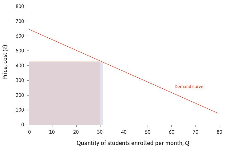
A person will buy the course if the price is less than or equal to their WTP. Suppose we line up the consumers in order of WTP, with the highest first, and plot a graph to show how the WTP varies along the line (Figure 7.5). You can see from the figure, for example, that at a price of Rs. 700, nobody would buy the course; if the course was offered for free, 100 people would sign up.
If we choose any price, say P = Rs. 220, Figure 7.5 shows the number of consumers whose WTP is greater than or equal to P. In this case, 60 consumers are willing to pay Rs. 220 or more, so the demand for LP’s course at a price of Rs. 220 is 60.
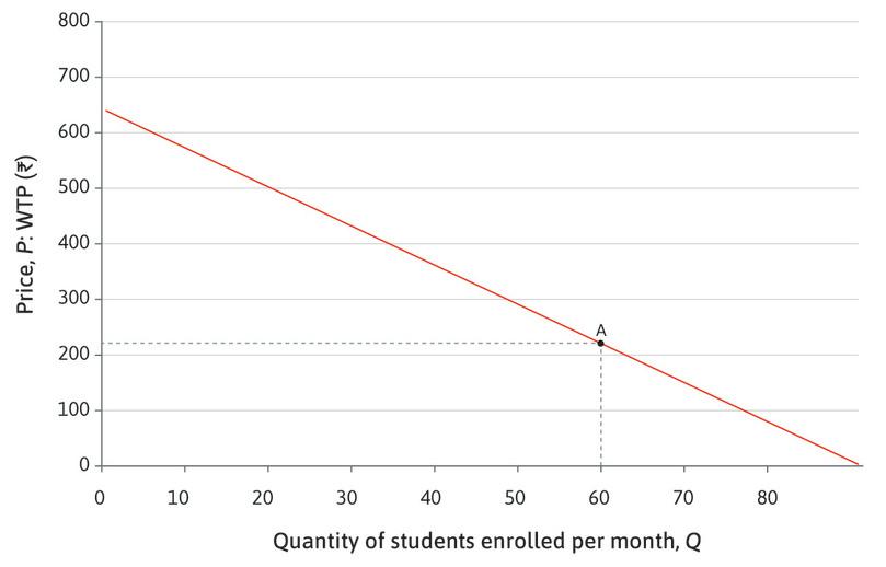
Figure 7.5 The demand for LP’s English course.
Because we have arranged the potential buyers in order of their WTP, it follows that if P is lower, there is a larger number of consumers willing to buy, so the demand is higher. Demand curves are often drawn as straight lines, as in this example, although there is no reason to expect them to be straight in reality—the demand curve for Apple Cinnamon Cheerios is not straight, for example. But we do expect demand curves to slope downward—as the price rises, the quantity demanded falls. In other words, when the available quantity is low, the course can be sold at a high price. This relationship between price and quantity is sometimes known as the law of demand.
The law of demand dates back to the seventeenth century and is attributed to Gregory King (1648–1712) and Charles Davenant (1656–1714). King was a herald at the College of Arms in London, who produced detailed estimates of the population and wealth of England. Davenant, a politician, published the Davenant-King law of demand in 1699, using King’s data. It described how the price of corn would change depending on the size of the harvest. For example, he calculated that a ‘defect’, or shortfall, of one-tenth (10%) would raise the price by 30%.
Price discrimination
- price discrimination
- A selling strategy in which different prices are set for different buyers or groups of buyers, or prices vary depending on the number of units purchased.
If you were the owner of the firm, LP, how would you choose the price for the English language course?
The first thought the owner might have is that she should go to the person with the greatest WTP and offer the course at a price slightly below that person’s WTP, ensuring that the person would buy. Then she would move on to the person with the next greatest WTP and offer the course at a price just below that customer’s WTP, and so on. This practice is called price discrimination. If the owner could do this, LP would make the most money possible from selling the English course to this population.
But price discrimination, at least the type that is finely tuned so that each individual pays a different price just below that customer’s WTP, is generally impossible. The seller has no way of determining the WTP of each potential buyer. The seller cannot find out by simply asking, because the potential buyer would often lie, so as to be able to buy the course at a lower price.
This particular concern is central to the story of ARVs that we mentioned earlier. While the multinational companies that sold the ARVs did offer them at a lower price to some African countries than to countries with developed economies, it would have been impossible to accurately find the willingness to pay for each buyer. In the pharmaceutical industry, another reason why substantial price discrimination is not the rule is that a buyer who purchased the course at a low price could then resell it to someone with a higher WTP, and end up making a profit. So, in this example someone could have bought the cheaper drugs at a lower price in some parts of Africa and resold them in the US for the market price there.
Some firms are able to practice a less individualized form of price discrimination by lowering prices for customers whose WTP might be less due to lower income, for example. Lower prices charged for students or the elderly are examples of price discrimination of this type. But for the most part, the product is sold at a single price to all customers.
Question 7.2 Choose the correct answer(s)
Figure 7.6 depicts two alternative demand curves, D and D′, for a product. Based on this graph, which of the following are correct?
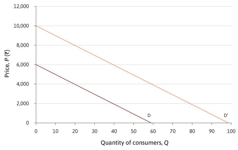
Figure 7.6 Two demand curves.
- On demand curve D, the firm can sell 10 units when the price is Rs. 5,000.
- When Q = 70, the corresponding price on D′ is Rs. 3,000.
- D′ can be seen as just a rightward shift of D, by 40 units—for any price, the firm can sell 40 more units on D′ than on D.
- With an output of 30 units, the firm can charge Rs. 4,000 more on D′ than on D.
7.3 Profits, costs, and the isoprofit curve
Imagining that you are the owner of a firm, your profits are the difference between sales revenue and production costs. So, before we can calculate profits, we need to know the production costs.
Let’s assume that LP is a very simple firm with a single owner. The company employs language teachers to design the English course. Production costs to the owner, per student, would be:
- Buying the raw materials: These cost Rs. 30 per student.
- The teachers’ time: Hiring the teachers costs Rs. 30 an hour, for ten hours.
- The owner’s time: We value this at what she would earn if she were employed elsewhere. We know that she could close her firm and get a job as a manager of someone else’s company making Rs. 60 an hour. She spends, on average, half an hour selling per student per course, so the opportunity cost of her time, per student, per course, would be Rs. 30.
Therefore, the cost to the owner, per student, per course, would be 30 + (30 × 10) + 30 = Rs. 360.
- constant returns to scale
- These occur when doubling all of the inputs to a production process doubles the output. The shape of a firm’s long-run average cost curve depends both on returns to scale in production and the effect of scale on the prices it pays for its inputs. See also: increasing returns to scale, decreasing returns to scale.
- unit cost
- Total cost divided by the number of units produced.
We assume that LP can simply hire more tutors and provide materials at the same costs, however many courses are offered (so the firm has constant returns to scale). Unit costs are constant at Rs. 360 for any level of the firm’s output (number of courses actually offered).
To maximize profit, the owner should produce exactly the quantity she expects to sell, and no more. Then revenue, costs, and profit are given by:
\[\begin{align*} \text{total costs} &= \text{unit cost} \times \text{quantity} \\ &= 360 \times Q \\ \text{total revenue} &= \text{price} \times \text{quantity} \\ &= P \times Q \\ \text{profit} &= \text{total revenue} − \text{total costs} \\ &= P \times Q - 360 \times Q \end{align*}\]So we have a formula for profit:
\[\text{profit} = (P−360) \times Q\]Using this formula, the owner can calculate the profit for any hypothetical combination of price and quantity.
- isoprofit curve
- A curve on which all points yield the same profit.
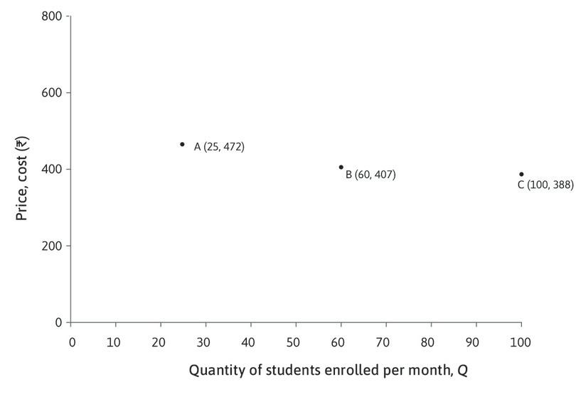
Work through the analysis of Figure 7.7 to see that there are many other combinations of price and number of courses sold per month that would give the owner profits of Rs. 2,800. The curve joining up all the combinations giving profits of Rs. 2,800 is called an isoprofit curve.
There will be an isoprofit curve where profits are zero—we have already seen that it is the average cost curve and it will be a horizontal line in Figure 7.7 at P = C = Rs. 360.
Just as indifference curves join points in a diagram that give the same level of utility, isoprofit curves join points that give the same level of total profit. Because it is the owner who gets the profits, we can think of the isoprofit curves as the owner’s indifference curves—the owner is indifferent between combinations of price and quantity that give her the same profit.
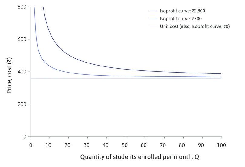
Figure 7.7 Isoprofit curves for the production of English courses.
Profit of Rs. 2,800
Other ways to make the same profit
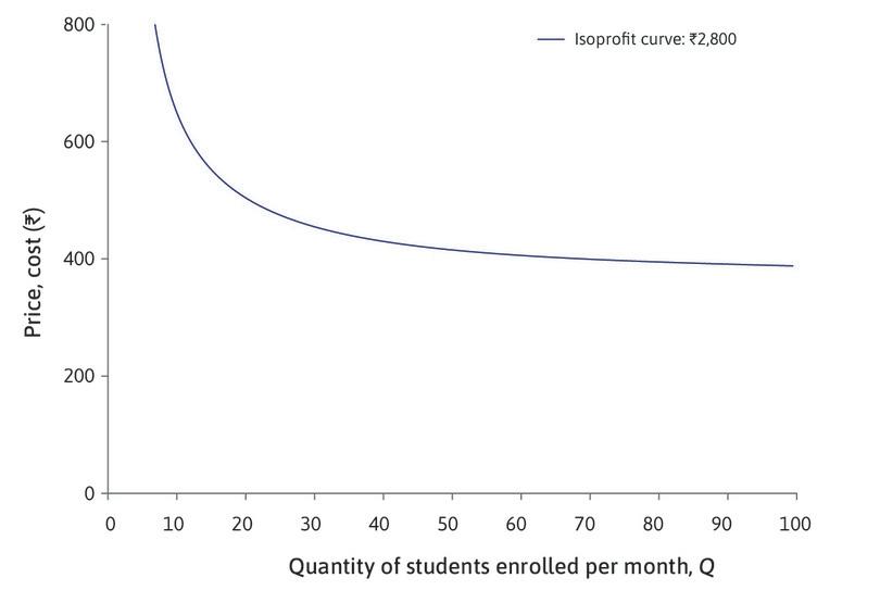
Isoprofit curve: Rs. 2,800
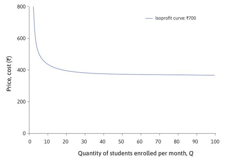
Isoprofit curve: Rs. 700
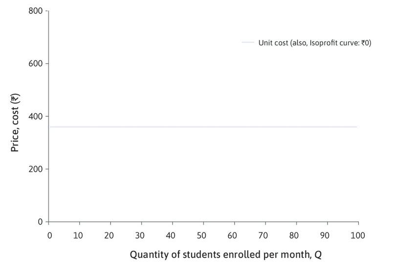
Zero-profit isocost curve—the average cost curve
Isoprofit curves
Question 7.3 Choose the correct answer(s)
A firm’s cost of production is Rs. 12 per unit of output. If P is the price of the output good and Q is the number of units produced, which of the following statements is correct?
- At (Q, P) = (2,000, 20), profit = (20 – 12) × 2,000 = Rs. 16,000.
- At (Q, P) = (1,200, 24), profit = (24 – 12) × 1,200 = Rs. 14,400. At (Q, P) = (2,000, 20), profit = (20 – 12) × 2,000 = Rs. 16,000. Therefore, (2,000, 20) is on a higher isoprofit curve.
- At (Q, P) = (2,000, 20), profit = (20 – 12) × 2,000 = Rs. 16,000. At (Q, P) = (4,000, 16), profit = (16 – 12) × 4,000 = Rs. 16,000. Therefore, these two points are on the same isoprofit curve.
- At P = 12 the firm makes no profit. Therefore (5,000, 12) will be on a horizontal isoprofit curve representing zero profit.
7.4 The isoprofit curves and the demand curve
To achieve a high profit, the owner would like both price and quantity to be as high as possible. She prefers points on higher isoprofit curves, but she is constrained by the demand curve. If she chooses a high price, she will be able to sell only a small quantity; if she wants to sell a large quantity, she must choose a low price.
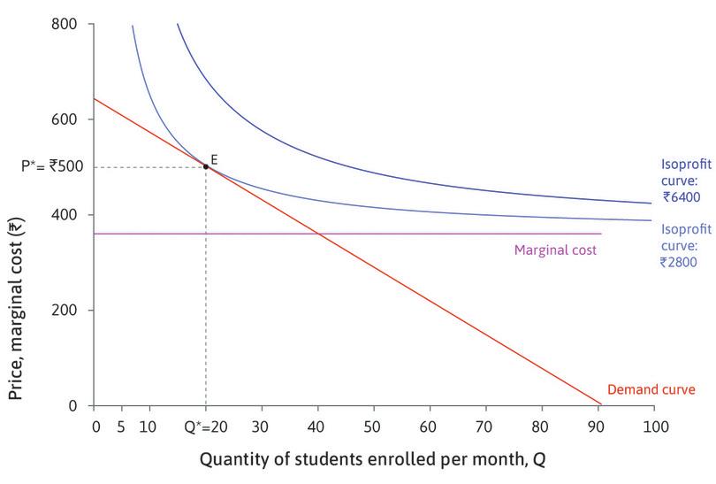
The demand curve determines what is feasible. Figure 7.8 shows the isoprofit curves and demand curve together. The owner faces a similar problem to Sakina, the weaver in Unit 3, who wanted to choose the point in her feasible set at which her utility was maximized. The owner should choose a feasible price and quantity combination that will maximize her profit.
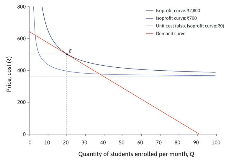
Figure 7.8 The profit-maximizing choice of price and quantity for English courses.
The profit-maximizing choice

Zero profits

Profit-maximizing choices
Maximizing profit at E
The owner’s best strategy is to choose point E in Figure 7.8; she should produce 20 courses and sell the course at a price of Rs. 500, making Rs. 2,800 profit. Just as in the case of Sakina in Unit 3, the optimal combination of price and quantity involves balancing two trade-offs:
- marginal rate of substitution (MRS)
- The trade-off that a person is willing to make between two goods. At any point, this is the slope of the indifference curve. See also: marginal rate of transformation.
- marginal rate of transformation (MRT)
- The quantity of some good that must be sacrificed to acquire one additional unit of another good. At any point, it is the slope of the feasible frontier. See also: marginal rate of substitution.
- The isoprofit curve is the owner’s indifference curve: Its slope at any point represents the trade-off she is willing to make between P and Q—her MRS. She would be willing to substitute a high price for a lower quantity if she obtained the same profit.
- The slope of the demand curve is the trade-off she is constrained to make: It is her MRT, or the rate at which the demand curve allows her to ‘transform’ quantity into price. She cannot raise the price without lowering the quantity, because fewer consumers will buy a more expensive product.
These two trade-offs balance at the profit-maximizing choice of P and Q.
The owner of LP probably didn’t think about the decision in this way.
Perhaps she remembered past experience in setting prices too low or too high (trial and error), or did some market research. However she made the choice, we expect that a firm could discover a profit-maximizing price and quantity. The purpose of our economic analysis is not to model the owner’s thought process to get to this point, but to understand the outcome when it does, and its relationship to the firm’s cost and consumer’s demand.
Question 7.4 Choose the correct answer(s)
The table represents market demand Q for a good at different prices P.
| Q | 100 | 200 | 300 | 400 | 500 | 600 | 700 | 800 | 900 | 1,000 |
| P | Rs. 270 | Rs. 240 | Rs. 210 | Rs. 180 | Rs. 150 | Rs. 120 | Rs. 90 | Rs. 60 | Rs. 30 | Rs. 0 |
The firm’s unit cost of production is Rs. 60. Based on this information, which of the following are correct?
- At Q = 100, profit = (270 − 60) × 100 = Rs. 21,000.
- At Q = 400, profit = (180 − 60) × 400 = Rs. 48,000. If you calculate the profit for each point on the demand curve you will see that profit is lower at the other points.
- The maximum profit is attained at Q = 400, where profit = (180 − 60) × 400 = Rs. 48,000.
- The firm will make a loss (negative profit) at all outputs above 800. At exactly 800, the profit is zero.
Question 7.5 Choose the correct answer(s)
Which of the following statements regarding the marginal rate of substitution (MRS) and the marginal rate of transformation (MRT) of a profit-maximizing firm are correct?
- The MRT is how much the firms have to drop the price for an incremental increase in demand. It is the slope of the demand curve.
- This is the definition of the MRS. It is the slope of the isoprofit curves.
- The MRT is the slope of the demand curve.
- When MRT > MRS, the slope of the demand curve is steeper than the slope of the isoprofit curve that intersects the demand curve. This means that, for a unit decrease in output, firms are able to increase the price more than the amount required to keep their profit constant. Therefore, to increase profit, they should decrease output.
Exercise 7.1 Changes in the market
Draw diagrams to show how the curves in Figure 7.8 would change in each of the following cases:
- A rival company producing a similar course slashes its prices.
- The cost of hiring producers for LPs’s course rises to Rs. 35 per hour (instead of Rs. 30).
- LP introduces a local advertising campaign costing Rs. 20 per minute.
In each case, explain what would happen to the price and the profit.
7.5 Looking at profit maximization through marginal revenue and marginal cost
In the previous section we showed that the profit-maximizing choice for LP was the point at which the demand curve was tangent to the highest isoprofit curve. To make maximum profit, it should sell Q = 20 courses at a price P = Rs. 500.
- marginal revenue
- The increase in revenue obtained by increasing the quantity from Q to Q + 1.
- marginal cost
- The effect on total cost of producing one additional unit of output. It corresponds to the slope of the total cost function at each point.
We now look at a different method of finding the profit-maximizing point, without using isoprofit curves. Instead, we use the marginal revenue curve and marginal cost curve. Remember that if Q courses are sold at a price P, revenue R is given by R = P × Q. The marginal revenue (MR) is the increase in revenue obtained by increasing the quantity from Q to Q + 1. Similarly if Q courses cost price C, cost C is given by C = C × Q. The marginal cost (MC) is the increase in cost incurred by increasing the quantity from Q to Q + 1. In our case, every additional unit costs the same (Rs. 360) and so the marginal cost is Rs. 360. The first unit costs Rs. 360, the first two cost Rs. 720. So the second unit costs Rs. 720 − Rs. 360 = Rs. 360. In this example, the marginal cost is constant, but it could actually change as production increased.
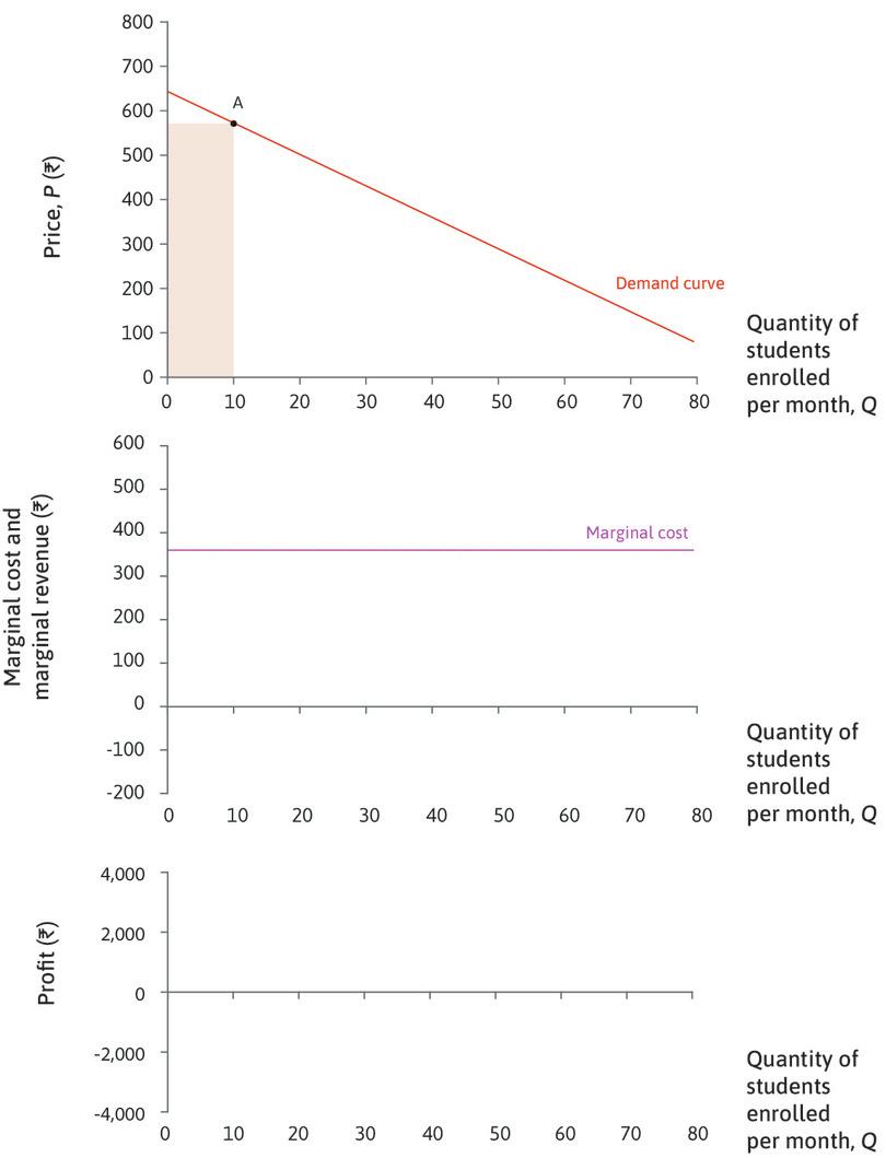
Figure 7.9a shows you how to calculate the marginal revenue when Q = 30: that is, the increase in revenue if quantity increases by one unit.
| Revenue, R = P × Q | ||
|---|---|---|
| Q = 30 | P = Rs. 430 | R = Rs. 12,900 |
| Q = 31 | P = Rs. 423 | R = Rs. 13,113 |
| ΔQ = 1 | ΔP = Rs. 7 | MR = ΔR/ΔQ = Rs. 213 |
| Gain in revenue (31st course) Loss of revenue (Rs. 7 on each of the other 30 courses) Marginal revenue |
Rs. 423 −Rs. 210 |
|
| Rs. 213 | ||
Figure 7.9a Calculating marginal revenue.
| Revenue, R = P × Q | ||
|---|---|---|
| Q = 30 | P = Rs. 430 | R = Rs. 12,900 |
| Q = 31 | P = Rs. 423 | R = Rs. 13,113 |
| ΔQ = 1 | ΔP = Rs. 7 | MR = ΔR/ΔQ = Rs. 213 |
| Gain in revenue (31st course) Loss of revenue (Rs. 7 on each of the other 30 courses) Marginal revenue |
Rs. 423 −Rs. 210 |
|
| Rs. 213 | ||
Revenue when Q = 30
| Revenue, R = P × Q | ||
|---|---|---|
| Q = 30 | P = Rs. 430 | R = Rs. 12,900 |
| Q = 31 | P = Rs. 423 | R = Rs. 13,113 |
| ΔQ = 1 | ΔP = Rs. 7 | MR = ΔR/ΔQ = Rs. 213 |
| Gain in revenue (31st course) Loss of revenue (Rs. 7 on each of the other 30 courses) Marginal revenue |
Rs. 423 −Rs. 210 |
|
| Rs. 213 | ||
Revenue when Q = 31

| Revenue, R = P × Q | ||
|---|---|---|
| Q = 30 | P = Rs. 430 | R = Rs. 12,900 |
| Q = 31 | P = Rs. 423 | R = Rs. 13,113 |
| ΔQ = 1 | ΔP = Rs. 7 | MR = ΔR/ΔQ = Rs. 213 |
| Gain in revenue (31st course) Loss of revenue (Rs. 7 on each of the other 30 courses) Marginal revenue |
Rs. 423 −Rs. 210 |
|
| Rs. 213 | ||
Marginal revenue when Q = 30

| Revenue, R = P × Q | ||
|---|---|---|
| Q = 30 | P = Rs. 430 | R = Rs. 12,900 |
| Q = 31 | P = Rs. 423 | R = Rs. 13,113 |
| ΔQ = 1 | ΔP = Rs. 7 | MR = ΔR/ΔQ = Rs. 213 |
| Gain in revenue (31st course) Loss of revenue (Rs. 7 on each of the other 30 courses) Marginal revenue |
Rs. 423 −Rs. 210 |
|
| Rs. 213 | ||
Why is MR > 0?
| Revenue, R = P × Q | ||
|---|---|---|
| Q = 30 | P = Rs. 430 | R = Rs. 12,900 |
| Q = 31 | P = Rs. 423 | R = Rs. 13,112 |
| ΔQ = 1 | ΔP = Rs. 7 | MR = ΔR/ΔQ = Rs. 213 |
| Gain in revenue (31st course) Loss of revenue (Rs. 7 on each of the other 30 courses) Marginal revenue |
Rs. 423 −Rs. 210 |
|
| Rs. 213 | ||
Calculating the marginal revenue
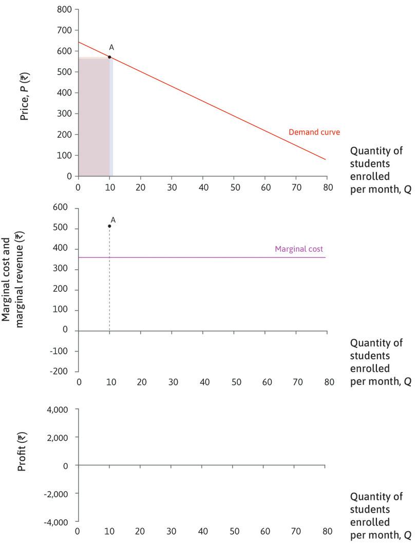
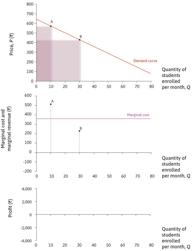
Figure 7.9a shows that the firm’s revenue is the area of the rectangle drawn below the demand curve. When Q is increased from 30 to 31, revenue changes for two reasons. An extra course is sold at the new price, but since the new price is lower when Q = 31, there is also a loss of Rs. 7 on each of the other 30 courses. The marginal revenue is the net effect of these two changes.
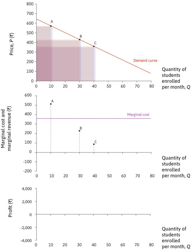
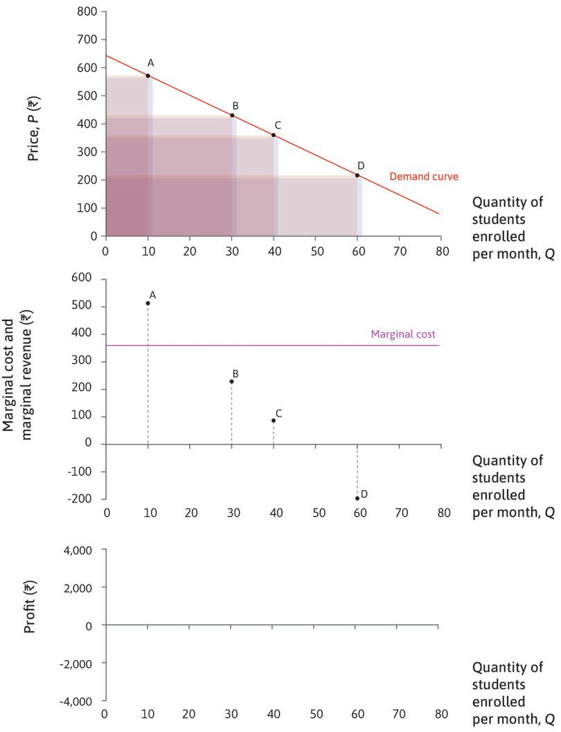
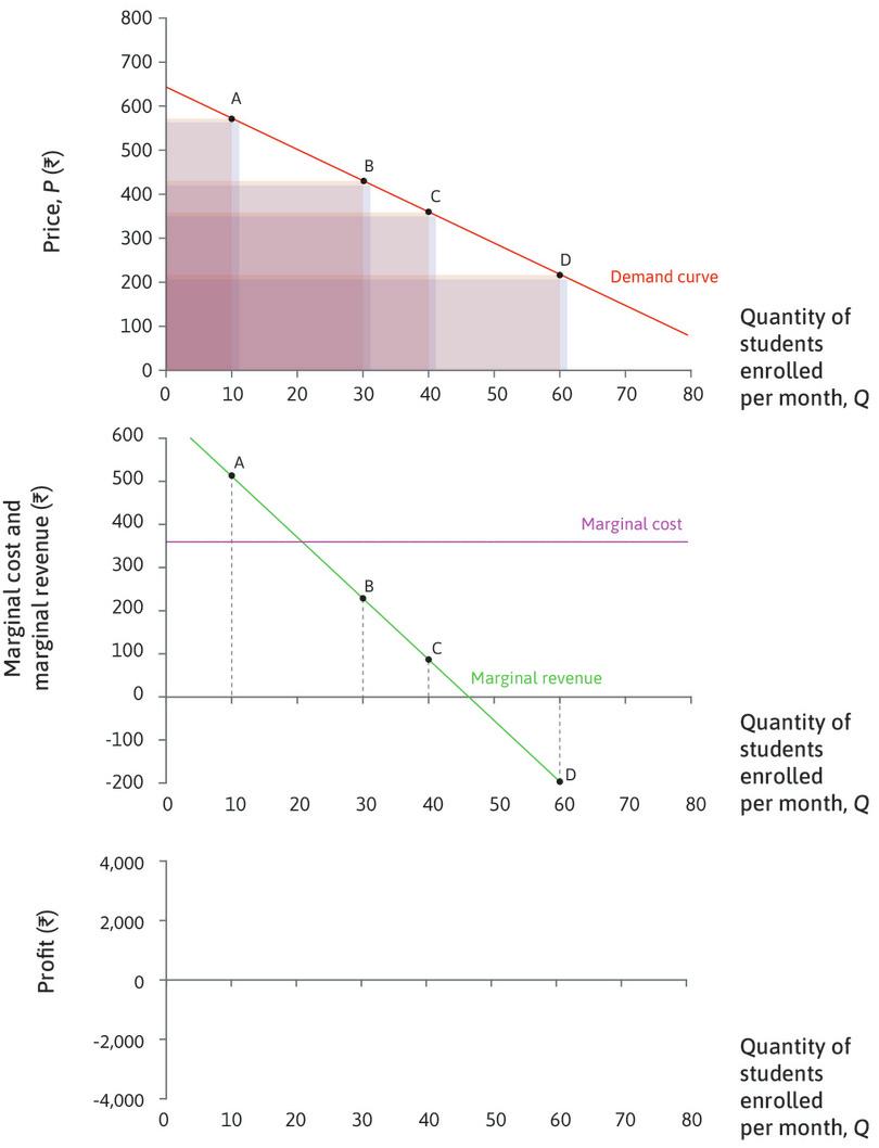
In Figure 7.9b we find the marginal revenue curve, and use it to find the point of maximum profit. The upper panel shows the demand curve. The middle panel shows the marginal cost curve: we know that the marginal cost of each course is Rs. 360, so the marginal cost curve is a horizontal line at a price of Rs. 360. The analysis in Figure 7.9b shows how to calculate and plot the marginal revenue curve. When P is high and Q is low, MR is high: the gain from selling one more course is much greater than the total loss on the small number of other courses. As we move down the demand curve P falls (so the gain on the last course gets smaller), and Q rises (so the total loss on the other courses is bigger), so MR falls and eventually becomes negative.
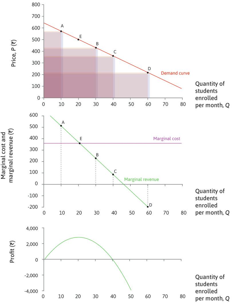
Figure 7.9b Marginal revenue, marginal cost, and profit.
Demand and marginal cost curves
Marginal revenue
Marginal revenue when Q = 30
Moving down the demand curve
MR < 0
The marginal revenue curve

MR > MC
MR < MC
The firm’s profit
The marginal revenue curve is usually (although not necessarily) a downward-sloping line. The lower two panels in Figure 7.9b demonstrate that the profit-maximizing point is where the MR curve crosses the MC curve. To understand why, remember that profit is the difference between revenue and costs, so for any value of Q, the change in profit if Q was increased by one unit (the marginal profit) would be the difference between the change in revenue, and the change in costs:
\[\begin{align*} \text{profit} &= \text{total revenue} - \text{total costs} \\ \text{marginal profit} &= \text{MR} - \text{MC} \end{align*}\]So:
- If MR > MC, the firm could increase profit by raising Q.
- If MR < MC, the marginal profit is negative. It would be better to decrease Q.
You can see how profit changes with Q in the lowest panel of 7.9b:
- When Q < 20, MR > MC: Marginal profit is positive, so profit increases with Q.
- When Q > 20, MR < MC: Marginal profit is negative; profit decreases with Q.
- When Q = 20, MR = MC: Profit reaches a maximum.
7.6 Gains from trade
- economic rent
- A payment or other benefit received above and beyond what the individual would have received in his or her next best alternative (or reservation option). See also: reservation option.
- total surplus
- The total gains from trade received by all parties involved in the exchange. It is measured as the sum of the consumer and producer surpluses.
- gains from exchange
- The benefits that each party gains from a transaction compared to how they would have fared without the exchange. Also known as: gains from trade. See also: economic rent.
Remember from Unit 5 that, when people engage voluntarily in an economic interaction, they do so because it makes them better off—they can obtain a surplus called economic rent, meaning the difference between how much they gain by this interaction compared to not engaging in the interaction. The total surplus for the parties involved is a measure of the gains from exchange (also known as gains from trade).
We can analyse the outcome of the economic interactions between consumers and a firm’s owner—just as we did for Angela and Bruno in Unit 5—and calculate the total surplus and the way it is shared.
We have assumed that the rules of the game for allocating English language courses to consumers are:
- A firm’s owner decides how many items to produce: The owner sets a single price at which admission to the course will be sold to all students.
- Then individual consumers decide whether to buy or not: No consumer buys more than one course.
In the interactions between a firm like Language Perfection and its consumers, there are potential gains for both the owner and the customers, as long as LP is able to produce courses at a cost less than its value to a consumer.
Recall that the demand curve shows the willingness to pay (WTP) of each of the potential consumers. A consumer whose WTP is greater than the price will buy the good and receive a surplus, since the value of the course to that customer is higher than the price.
- consumer surplus
- The consumer’s willingness to pay for a good minus the price at which the consumer bought the good, summed across all units sold.
- producer surplus
- The price at which a firm sells a good minus the minimum price at which it would have been willing to sell the good, summed across all units sold.
And if the price paid by the customer is greater than what it costs the firm to offer the course, the owner receives a surplus too. This surplus is higher than the amount the owner would earn as a manager in another company, which we have included in the cost of producing the course. Figure 7.10 shows how to find the total surplus for the firm and its consumers, when LP sets the price to maximize its profits.
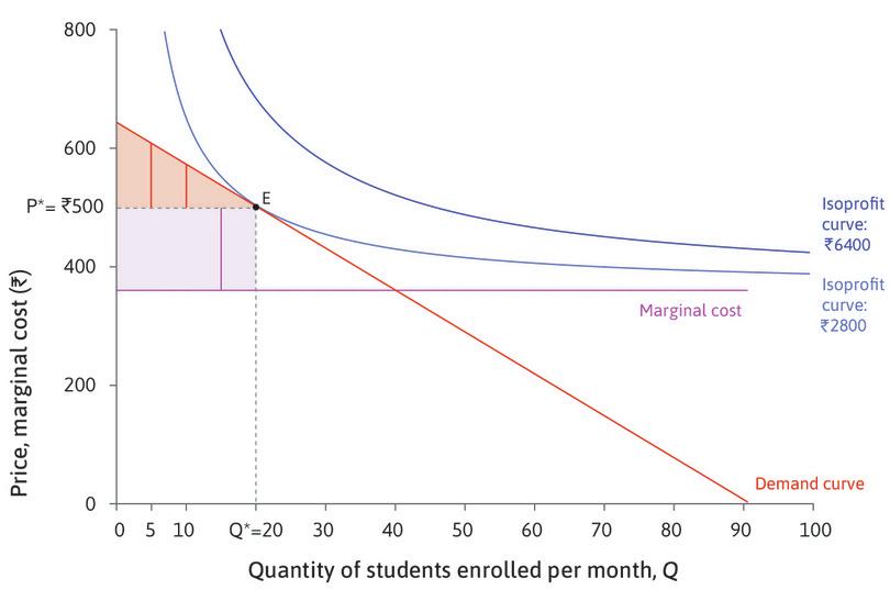
Figure 7.10 Gains from trade.
The firm set its profit-maximizing price
A higher WTP

What would the tenth customer have been willing to pay?

The consumer surplus
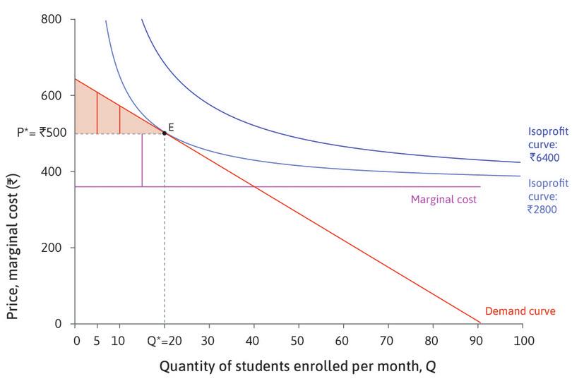
The producer surplus on a single lesson
The total producer surplus
In Figure 7.10, the shaded area above P* measures the consumer surplus, and the shaded area below P* is the producer surplus. We see from the relative size of the two areas in Figure 7.10 that, in this market, the firm obtains a greater share of the surplus.
As in the voluntary contracts between Angela and Bruno in Unit 5, both parties gain in the market for language courses. The division of the gains is determined by bargaining power. In this case, the firm is the only seller of this course, and can set a high price and obtain a high share of the gains, knowing that those who value the course highly have no alternative but to accept. The firm has many other potential customers, and so people have no power to bargain for a better deal.
Consumer surplus, producer surplus, and profit
- The consumer surplus is a measure of the benefits of participation in the market for consumers.
- The producer surplus is closely related to the firm’s profit. In our example they are exactly the same thing, but that is because we have assumed that the firm doesn’t have any fixed costs.
- In general, the profit is equal to the producer surplus minus the firm’s fixed costs. The firm LP would have fixed costs if, for example, it paid for advertising for its courses.
- The total surplus arising from trade in this market, for the firm and consumers together, is the sum of consumer and producer surplus.
Evaluating the outcome using the Pareto efficiency criterion
- Pareto efficient
- An allocation with the property that there is no alternative technically feasible allocation in which at least one person would be better off, and nobody worse off.
Is the allocation of language courses in this market Pareto efficient? To answer this question, we need to know all the technically feasible outcomes. These are combinations of price and quantity on the demand curve, where the price is no lower than the cost of production. If there is another technically feasible outcome in which at least one person (customer or owner) is better off and no one is worse off, then the outcome is not Pareto efficient.
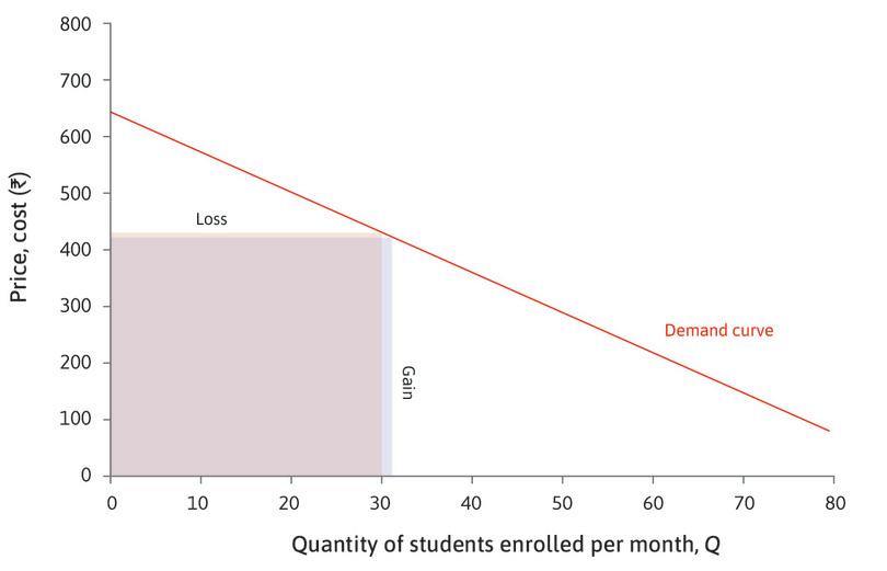
Beginning at the allocation E in Figure 7.10 and considering the customers, it is clear that there are some consumers who do not purchase the course at the firm’s chosen price, but who would nevertheless be willing to pay more than it would cost the firm to produce the course, namely Rs. 360.
- Pareto improvement
- A change that benefits at least one person without making anyone else worse off. See also: Pareto dominant.
But we also know that, at any price below Rs. 500 (the profit-maximizing price at point E), profits are lower (the owner would be on an isoprofit curve with lower profits). It appears that a Pareto improvement is not possible because, although consumers would be better off, the owner would be worse off.
But evaluating whether the outcome is Pareto efficient does not mean the rules of the game must be kept unchanged. If there is a technically feasible allocation in which at least one person is better off and nobody is worse off, then E is not Pareto efficient.
If LP could practise price discrimination, it could offer one more language course and sell it to the 21st consumer at a price lower than Rs. 500 but higher than the production cost. (The other 20 customers would continue to pay Rs. 500.) This would be a Pareto improvement—both the firm and the 21st consumer would be better off; the other 20 would be no worse off. The firm’s profit on the 21st course sold would be lower than on the 20th but total profits would rise. Remember that the isoprofit curve is drawn assuming that all customers pay the same price. We need to add the profit on the 21st course to Rs. 2,800 to calculate the firm’s total profits.
The 21st consumer benefits from being able to buy the language course.
This example shows that the potential gains from trade in the market for this type of language course have not been exhausted at E.
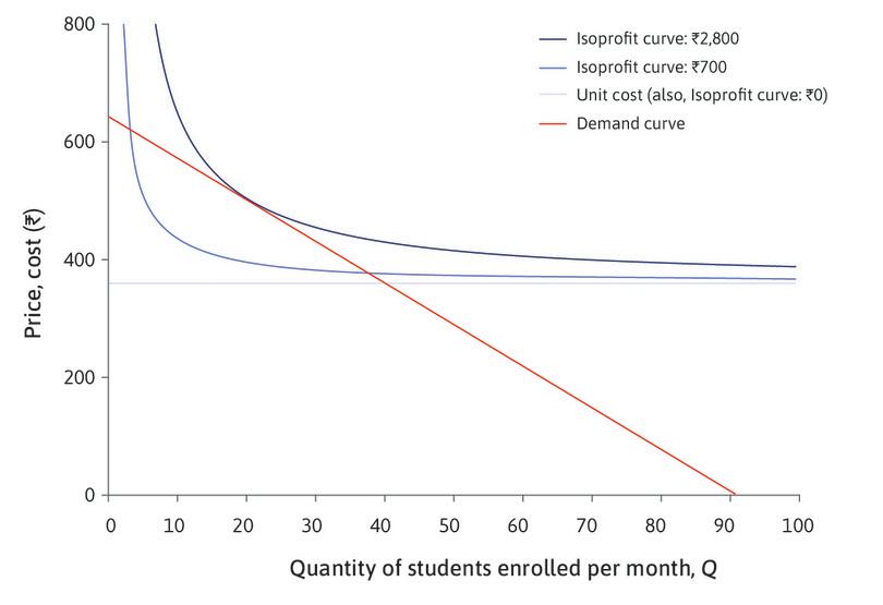
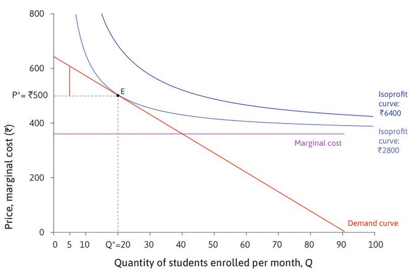
In Figure 7.11 we have drawn the demand curve again, as well as the marginal cost line, which is a horizontal line at Rs. 360. Look at point F, where the two lines cross. You can see that the fortieth consumer has a WTP that is equal to the marginal cost of a course. For the thirty-ninth consumer, the WTP exceeds the cost, so not offering the forty-second course would not be efficient. For the forty-first consumer, the WTP is less than the cost, so offering more than 40 courses would also not be efficient.
Figure 7.11 shows that the total surplus, which we can think of as the pie to be shared between the owner and LP’s customers, would be the highest possible if the firm produced 40 courses and sold them for Rs. 360.
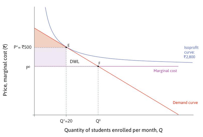
Figure 7.11 Deadweight loss.
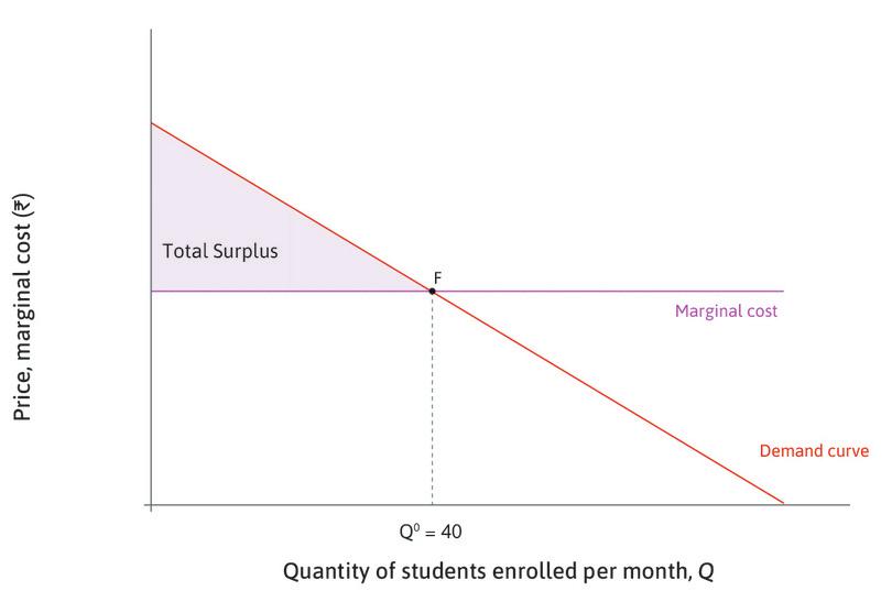
The total surplus at F
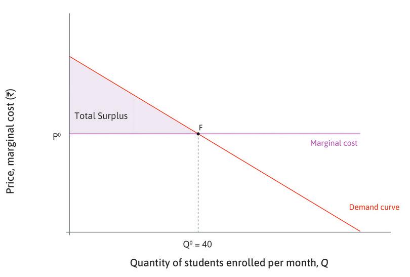
Producing at F would be Pareto efficient
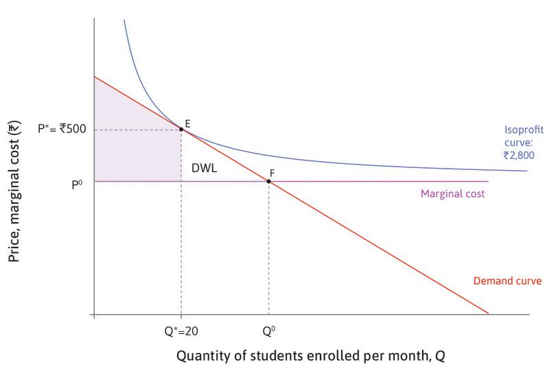
The total surplus at E is smaller
The division of the surplus at E
- deadweight loss
- A loss of total surplus relative to a Pareto-efficient allocation.
Since the firm chooses E rather than F, there is a loss of potential surplus, known as the deadweight loss.
It might seem confusing that the firm chooses E when we said that, at this point, it would be possible for both the consumers and the owner to be better off. That is true, but only if LP could practise price discrimination by selling courses to other consumers at a lower price than to the first 20 consumers. The owner chooses E because that is the best she can do given the rules of the game (setting one price for all consumers). To sell 40 courses without price discrimination, she would have to set a price of Rs. 360, so her profits would be zero.
The allocation that results from price-setting by the producer of a differentiated product like LP’s language course is Pareto inefficient. The owner uses the firm’s bargaining power to set a price that is higher than the marginal cost of a course. The firm keeps the price high by producing a quantity that is too low, relative to the Pareto-efficient allocation.
Exercise 7.2 shows that, in an unlikely scenario in which the firm could engage in price discrimination and charge different prices for each buyer, it would be possible to achieve a Pareto-efficient allocation.
Exercise 7.2 Changing the rules of the game
- Suppose that LP had sufficient information and enough bargaining power to charge each individual consumer the maximum they would be willing to pay. Draw the demand curve and marginal cost line (as in Figure 7.11), and indicate on your diagram:
- the number of courses sold
- the highest price paid by any consumer
- the lowest price paid by any consumer
- the consumer and producer surplus.
- Give examples of goods that are sold in this way.
- Why is price discrimination not common practice? Explain your reasons.
- Some firms charge different prices to different groups of consumers, for example, airlines may charge higher fares for last-minute travellers. Why would they do this, and what effect would it have on the consumer and producer surpluses?
- Now suppose that price discrimination is impossible, and that it becomes very easy for language firms to set up in the city in which LP operates. How could this give consumers more bargaining power?
- Under these rules, how many courses would be sold?
- Under these rules, what would the producer and consumer surpluses be?
Question 7.6 Choose the correct answer(s)
Which of the following statements are correct?
- To be more precise, each consumer receives a surplus equal to the difference between the WTP and the price, and consumer surplus is the sum of the surpluses of all consumers.
- Producer surplus is the difference between the firm’s revenue and its marginal costs. This is not the same as profit, because—unlike the case of the firm LP—there may be fixed costs of production. The profit is the producer surplus minus the fixed costs.
- The deadweight loss is the loss of potential total surplus due to the firm producing below the Pareto-efficient level. It is the sum of the surplus losses of both the consumers and the producer.
- All possible gains would be achieved at the Pareto-efficient output level. But the profit-maximizing choice of a firm producing a differentiated good is not Pareto efficient.
7.7 The elasticity of demand
The firm maximizes profit by choosing the point where the slope of the isoprofit curve (MRS) is equal to the slope of the demand curve (MRT), which represents the trade-off that the firm is constrained to make between price and quantity.
- price elasticity of demand
- The percentage change in demand that would occur in response to a 1% increase in price. We express this as a positive number. Demand is elastic if this is greater than 1, and inelastic if less than 1.
So the firm’s decision depends on how steep the demand curve is: in other words, how much consumers’ demand for a good will change if the price changes. The price elasticity of demand is a measure of the responsiveness of consumers to a price change. It is defined as the percentage change in demand that would occur in response to a 1% increase in price. For example, suppose that when the price of a product increases by 10%, we observe a 5% fall in the quantity sold. Then we calculate the elasticity, ε, as follows:
\[\varepsilon = -\frac{\% \text{ change in demand}}{\% \text{ change in price}}\]ε is the Greek letter epsilon, which is often used to represent elasticity. For a demand curve, quantity falls when price increases. So the change in demand is negative if the price change is positive, and vice versa. The minus sign in the formula for the elasticity ensures that we get a positive number as our measure of responsiveness. So in this example we get:
\[\begin{align} \varepsilon &= -\frac{-5}{10} \\ &= 0.5 \end{align}\]The price elasticity of demand is related to the slope of the demand curve. If the demand curve is quite flat, the quantity changes a lot in response to a change in price, so the elasticity is high. Conversely, a steeper demand curve corresponds to a lower elasticity. But they are not the same thing, and it is important to notice that the elasticity changes as we move along the demand curve, even if the slope doesn’t.
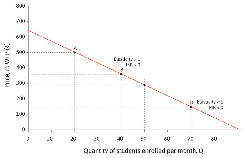
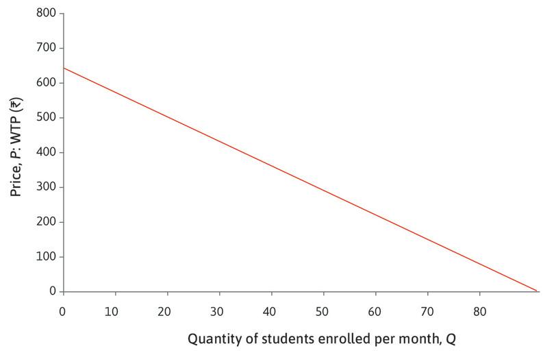
Figure 7.12 shows (again) the demand curve for language courses, which has a constant slope: it is a straight line. At every point, if the quantity increases by one (ΔQ = 1), the price falls by Rs. 7 (ΔP = –Rs. 7):
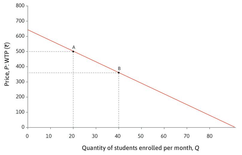
\[\begin{align*} \text{slope of the demand curve} &= -\frac{\Delta P}{\Delta Q} \\ &= -7 \end{align*}\]Since ΔP = −Rs. 7 when ΔQ = 1 at every point on the demand curve, it is easy to calculate the elasticity at any point. At A, for example, Q = 20 and P = Rs. 500. So:
\[\begin{align*} \%\text{ change in }Q &= 100(\frac{\Delta Q}{Q}) = 100(\frac{1}{20}) = 5\% \\ \%\text{ change in }P &= 100(\frac{\Delta P}{P}) = 100(\frac{-7}{500}) = -1.4\% \end{align*}\]And so:
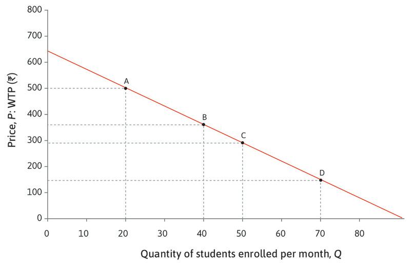
\[\begin{align*} \varepsilon &= -\frac{5}{-1.4} \\ &= 3.57 \end{align*}\]The table in Figure 7.12 calculates the elasticity at several points on the demand curve. Use the steps in the analysis to see that, as we move down the demand curve, the same changes in P and Q lead to a higher percentage change in P and a lower percentage change in Q, so the elasticity falls.
| Elasticity = − % Change in Q/% Change in P | ||||
|---|---|---|---|---|
| A | B | C | D | |
| Q | 20 | 40 | 50 | 70 |
| P | Rs. 500 | Rs. 360 | Rs. 290 | Rs. 150 |
| ΔQ | 1 | 1 | 1 | 1 |
| ΔP | −Rs. 7 | −Rs. 7 | −Rs. 7 | −Rs. 7 |
| % change in Q | 5.00 | 2.50 | 2.00 | 1.43 |
| % change in P | −1.40 | −1.94 | −2.41 | −4.11 |
| Elasticity | 3.57 | 1.29 | 0.83 | 0.34 |
| MR | Rs. 367 | Rs. 87 | -Rs. 53 | -Rs. 333 |
Figure 7.12 The elasticity of demand for courses.
| Elasticity = − % Change in Q/% Change in P | ||||
|---|---|---|---|---|
| A | B | C | D | |
| Q | 20 | 40 | 50 | 70 |
| P | Rs. 500 | Rs. 360 | Rs. 290 | Rs. 150 |
| ΔQ | 1 | 1 | 1 | 1 |
| ΔP | −Rs. 7 | −Rs. 7 | −Rs. 7 | −Rs. 7 |
| % change in Q | 5.00 | 2.50 | 2.00 | 1.43 |
| % change in P | −1.40 | −1.94 | −2.41 | −4.66 |
| Elasticity | 3.57 | 1.29 | 0.83 | 0.34 |
| MR | Rs. 367 | Rs. 87 | -Rs. 53 | -Rs. 333 |
Elasticity at A
| Elasticity = − % Change in Q/% Change in P | ||||
|---|---|---|---|---|
| A | B | C | D | |
| Q | 20 | 40 | 50 | 70 |
| P | Rs. 500 | Rs. 360 | Rs. 290 | Rs. 150 |
| ΔQ | 1 | 1 | 1 | 1 |
| ΔP | −Rs. 7 | −Rs. 7 | −Rs. 7 | −Rs. 7 |
| % change in Q | 5.00 | 2.50 | 2.00 | 1.43 |
| % change in P | −1.40 | −1.94 | −2.41 | −4.66 |
| Elasticity | 3.57 | 1.29 | 0.83 | 0.34 |
| MR | Rs. 367 | Rs. 87 | -Rs. 53 | -Rs. 333 |
Elasticity is lower at B than at A
| Elasticity = − % Change in Q/% Change in P | ||||
|---|---|---|---|---|
| A | B | C | D | |
| Q | 20 | 40 | 50 | 70 |
| P | Rs. 500 | Rs. 360 | Rs. 290 | Rs. 150 |
| ΔQ | 1 | 1 | 1 | 1 |
| ΔP | −Rs. 7 | −Rs. 7 | −Rs. 7 | −Rs. 7 |
| % change in Q | 5.00 | 2.50 | 2.00 | 1.43 |
| % change in P | −1.40 | −1.94 | −2.41 | −4.66 |
| Elasticity | 3.57 | 1.29 | 0.83 | 0.34 |
| MR | Rs. 367 | Rs. 87 | -Rs. 53 | -Rs. 333 |
As Q increases, elasticity decreases
| Elasticity = − % Change in Q/% Change in P | ||||
|---|---|---|---|---|
| A | B | C | D | |
| Q | 20 | 40 | 50 | 70 |
| P | Rs. 500 | Rs. 360 | Rs. 290 | Rs. 150 |
| ΔQ | 1 | 1 | 1 | 1 |
| ΔP | −Rs. 7 | −Rs. 7 | −Rs. 7 | −Rs. 7 |
| % change in Q | 5.00 | 2.50 | 2.00 | 1.43 |
| % change in P | −1.40 | −1.94 | −2.41 | −4.66 |
| Elasticity | 3.57 | 1.29 | 0.83 | 0.34 |
| MR | Rs. 367 | Rs. 87 | -Rs. 53 | -Rs. 333 |
The marginal revenue
We say that demand is elastic if the elasticity is higher than 1, and inelastic if it is less than 1. You can see from the table in Figure 7.12 that the marginal revenue is positive at points where demand is elastic, and negative where it is inelastic. Why does this happen? When demand is highly elastic, price will only fall a little if the firm increases its quantity. So by producing one extra course, the firm will gain revenue on the extra course without losing much on the other courses and total revenue will rise; in other words, MR > 0. Conversely, if demand is inelastic, the firm cannot increase Q without a big drop in P, so MR < 0. In the Einstein at the end of this section, we demonstrate that this relationship is true for all demand curves.
Question 7.7 Choose the correct answer(s)
A shop sells 20 hats per week at Rs. 10 each. When it increases the price to Rs. 12, the number of hats sold falls to 15 per week. Which of the following statements are correct?
- When the price increases from Rs. 10 to Rs. 12, demand decreases.
- The percentage price increase is 100 × 2/10 = 20%. It causes a percentage decrease in demand of 100 × 5/20 = 25%.
- Using the figures to estimate the price elasticity of demand gives a value greater than 1, so demand is elastic.
- The percentage price increase is 100 × 2/10 = 20%; the percentage decrease in demand is 100 × 5/20 = 25%. So the elasticity can be estimated as 25/20 = 1.25.
How does the elasticity of demand affect a firm’s decisions? Remember that the LP’s profit-maximizing quantity is Q = 20. You can see in Figure 7.12 that this is on the elastic part of the demand curve. The firm would never want to choose a point such as D where the demand curve is inelastic because the marginal revenue is negative there; it would always be better to decrease the quantity, since that would raise revenue and decrease costs. So the firm always chooses a point where the elasticity is greater than 1.
- profit margin
- The difference between the price and the marginal cost.
Secondly, the firm’s profit margin (the difference between the price and the marginal cost of production) is closely related to the elasticity of demand. Figure 7.13 represents a different situation of highly elastic demand. The demand curve is quite flat, so small changes in price make a big difference to sales. The profit-maximizing choice is point E. You can see that the profit margin is relatively small.
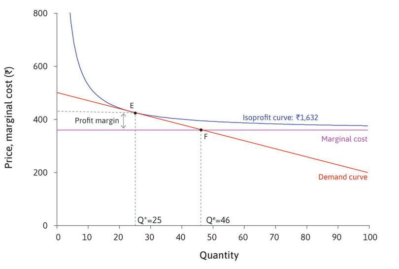
Figure 7.13 A firm facing highly elastic demand.
Figure 7.14 shows the decision of a firm with the same costs of course production, but less elastic demand for its product. In this case, the profit margin is high, and the quantity is low. When the price is raised, many consumers are still willing to pay. The firm maximizes profits by exploiting this situation, obtaining a higher share of the surplus. In both cases, the profit-maximizing output (point E), is around half of the pareto-efficient output (point F). However, in the second case, the profit margin is much higher.
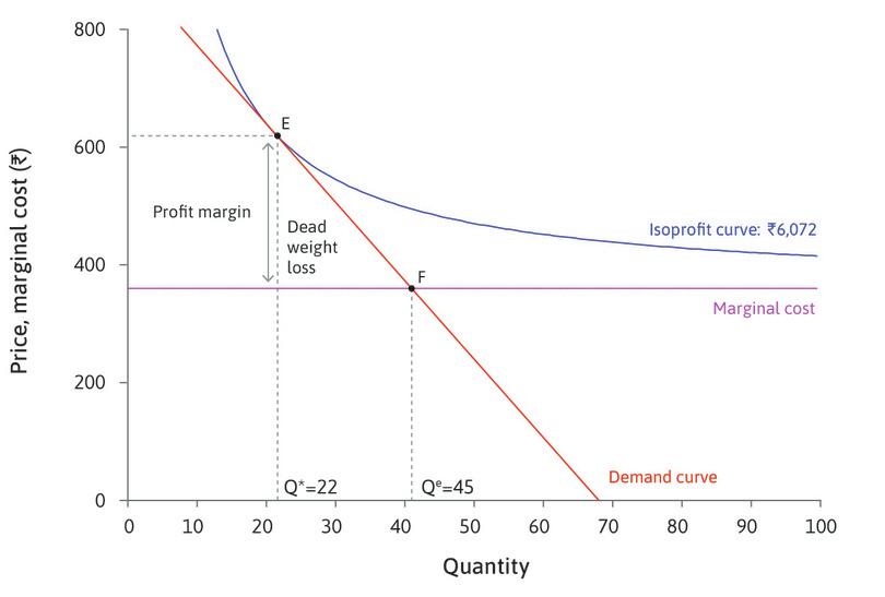
Figure 7.14 A firm facing less elastic demand.
- price markup
- The price minus the marginal cost divided by the price. It is inversely proportional to the elasticity of demand for this good.
Leibniz: The elasticity of demand
These examples illustrate that the lower the elasticity of demand, the more the firm will raise the price above the marginal cost to achieve a high profit margin. When demand elasticity is low, the firm has the power to raise the price without losing many customers, and the markup, which is the profit margin as a proportion of the price, will be high. The Einstein at the end of this section shows you that the markup is inversely proportional to the elasticity of demand.
Question 7.8 Choose the correct answer(s)
The figure depicts two demand curves, D1 and D2.
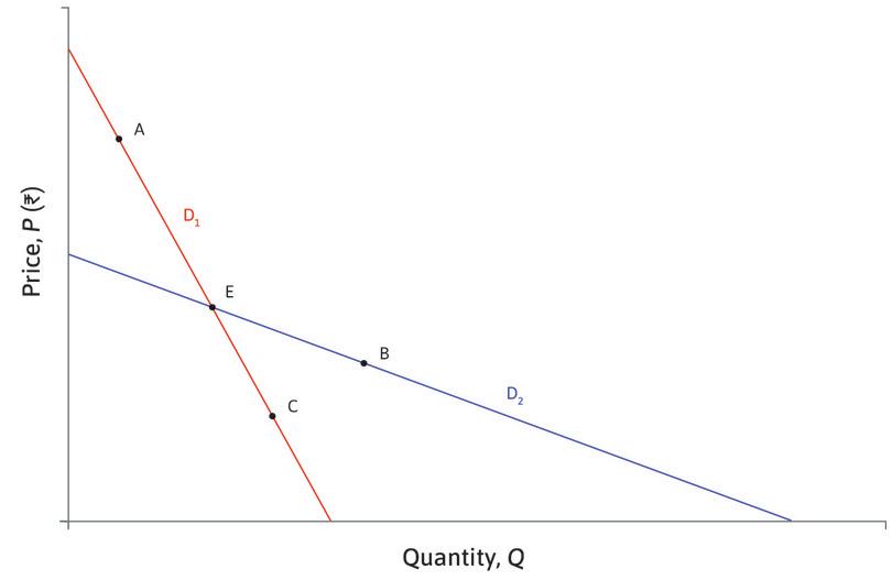
Based on this figure, which of the following statements are correct?
- At E, the price and quantity are the same on both demand curves, but D1 is steeper, so it is less elastic than D2.
- The slope is the same at A and C, but at A the price is higher and quantity is lower, so the elasticity is higher.
- The price and quantity are the same on both demand curves, but D1 is steeper, so the elasticities are not the same.
- The slope is the same at E and C. But at E the price is higher and quantity is lower, so the elasticity is higher.
Einstein The elasticity of demand and the marginal revenue
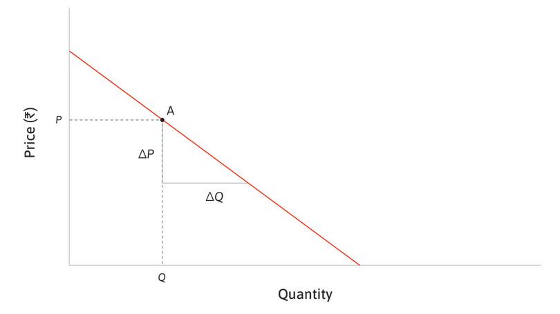
The diagram shows how to obtain a general formula for the elasticity at a point (Q, P) on the demand curve.
It also shows how the elasticity is related to the slope of the demand curve. A flatter demand curve has a lower slope, indicating higher elasticity.
![The elasticity of demand and the marginal revenue.]()
Figure 7.15 The elasticity of demand and the marginal revenue.
At point A, the price is P and the quantity is Q. If the quantity increases by ΔQ, the price falls: it changes by ΔP, which is negative.
\[\begin{align*} \text{% change in } P = 100 \times \Delta P/P \\ \text{% change in } Q = 100 \times \Delta Q/Q \\ \text{Elasticity at A} = -\frac{\text{ % change in }Q}{\text{% change in } P} \\ = - \frac{\Delta Q/Q}{\Delta P/P} \\ = - \frac{P}{Q} \times \frac{\Delta Q}{\Delta P} \\ \text{slope of demand curve} = \frac{\Delta P}{\Delta Q} \\ \text{Elasticity} = - \frac{P}{Q} \times \frac{1}{slope} \end{align*}\]Suppose that the demand curve is elastic at A. Then the elasticity is greater than one:
\[-\frac{P \Delta Q}{Q \Delta P} > 1\]Multiplying by −QΔP (which is positive):
\[P\Delta Q > -Q\Delta P\]and rearranging, we get:
\[P\Delta Q + Q\Delta P > 0\]Consider the special case when ΔQ = 1. The inequality becomes:
\[P + Q \Delta P > 0\]Now remember that the marginal revenue at point A is the change in revenue when Q increases by one unit. This change consists of the gain in revenue on the extra unit, which is P, and the loss on the other units, which is QΔP. So this inequality tells us that the marginal revenue is positive.
We have shown that if the demand curve is elastic, MR > 0. Similarly, if the demand curve is inelastic, MR < 0.
The size of the markup chosen by the firm
We can find a formula that shows that the markup is high when the elasticity of demand is low.
We know that the firm chooses a point where the slope of the isoprofit curve is equal to the slope of the demand curve, and that the slope of the demand curve is related to the price elasticity of demand:
\[\varepsilon = -\frac{P}{Q}\times\frac{1}{\text{slope}}\]Rearranging this formula:
\[\text{slope of demand curve} = -\frac{P}{Q}\times\frac{1}{\text{elasticity}}\]We also know from Section 7.3:
\[\text{slope of isoprofit curve} = -\frac{(P- \text{MC})}{Q}\]When the two slopes are equal:
\[\frac{(P - \text{MC})}{Q} = \frac{P}{Q}\times\frac{1}{\text{elasticity}}\]Rearranging this gives us:
\[\frac{(P - \text{MC})}{P} = \frac{1}{\text{elasticity}}\]The left-hand side is the profit margin as a proportion of the price, which is called the markup. Therefore:
The firm’s markup is inversely proportional to the elasticity of demand.
7.8 Costs and Output
- average cost
- The total cost of the firms’s output divided by the total number of units of output.
In the example of LP, the marginal cost was fixed at Rs. 360. Whatever number of units were sold, the cost of each unit was the same. We can also define the average cost as the total cost of production divided by the quantity of output produced or sold. Because in this case every unit costs the same, the average cost is the same as the marginal cost. If it sold 4 courses, the total cost would be Rs. 1440 ÷ 4 = Rs. 360. But this need not be true across all firms and production techniques.
Recall our discussion on fixed costs early on in this unit. We saw that firms making products requiring R&D incur significant fixed costs–this is true in the case of the ARVs as well. Producing the first unit of the drug cost a great deal since it included the cost of research and development, testing, and setting up of the factory. But once this initial cost was incurred, every other unit sold cost much less since it would only include raw material and labour costs and not the cost of R&D. So in this case, the average cost of production would have fallen as more and more units were produced. This is true across many different sorts of firms. Software products are another example of this—consider how much the first copy of Microsoft Word might have cost and how much each subsequent copy did.
It is also possible that as output increases, some firms get better at production so that each additional unit of output actually costs less, i.e. marginal costs diminish. One reason for this may be that firms learn how to produce more efficiently the more they produce (this is sometimes called ‘learning by doing’).
There is one more possibility: consider the copper mining industry. Assume there is a company which has bought several mines. It may begin by extracting copper from the highest yielding mine so that the cost per unit is low, but once exhausted it has to move to another mine where it costs more to obtain the same amount of copper. Consequently, the cost of mining a particular amount of copper actually rises as production increases. In this case, the firm faces a rising marginal cost curve.
If there are fixed costs, and the marginal cost is constant, the firm faces falling average costs as more and more output is being produced at the same cost per additional unit. Similarly, if marginal costs are falling, then the average cost will also fall, as it is cheaper to produce more units of output. However, if marginal cost is rising, then the total cost of production increases at an increasing rate. Hence, the average cost first falls, and then rises. Work through Figure 7.16 to see how total cost, average cost, and marginal costs change with different kinds of firms.
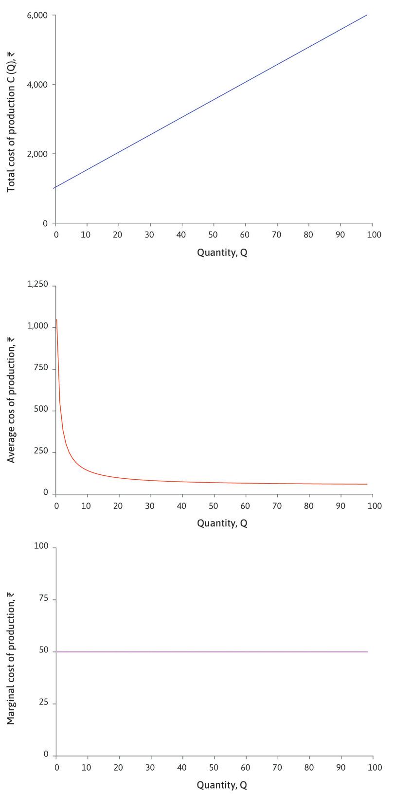
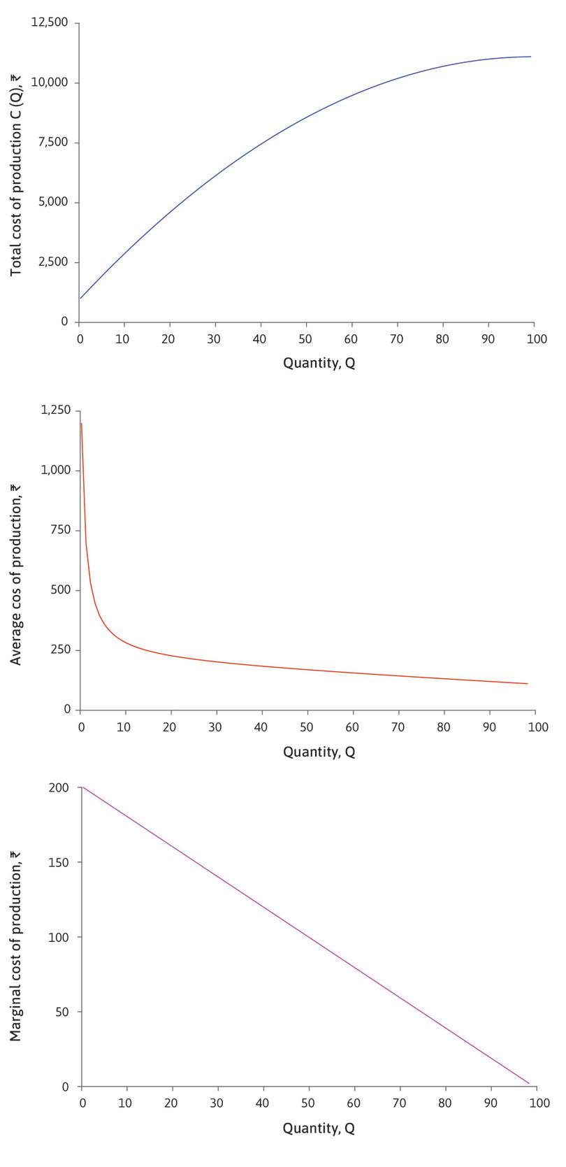
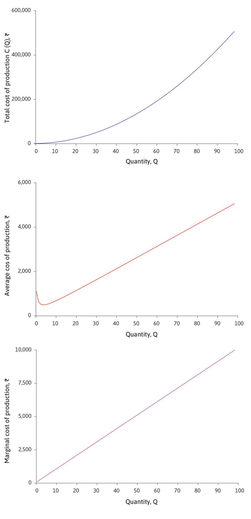
Figure 7.16 Cost curves for different kinds of firms
Firms with high fixed cost and constant marginal cost
Firms with falling marginal cost
Firms with rising marginal costs
How economists learn from facts Using surveys to understand marginal costs
One advantage social scientists have over natural scientists is that they can ask their subjects about their behaviour and often get useful responses. For example, surveys and questionnaires are often used by economists to try and understand economic behaviour and outcomes.
In 1991, Alan Blinder, a Princeton economist, did exactly this. He approached a national, multi-industry sample of industry leaders to ask them about their pricing decisions and what their cost structure looked like. He found several interesting results. Of the 200 executives interviewed, nearly half of them (48%) claimed that marginal costs were constant in their firm. About 40% suggested that their marginal costs were declining. Finally, about 11% suggested that their firms faced rising marginal costs.6
Exercise 7.3 How much does the COVID-19 vaccine cost?
Read this article on COVID-19 vaccine pricing by Abhishek De. The author discusses various possible vaccines that are in development by various pharmaceutical companies to fight the coronavirus pandemic, and the prices at which these companies will be offering the vaccine courses to consumers across the world. Answer the following questions.
- In 2019, how much were Oxford University and Pfizer spending to develop their respective vaccines (in $)?
- At what price were they aiming to sell the vaccine?
- Why is there such a huge gap in the cost incurred by these companies and the price at which the vaccines are sold?
- Draw the shape of the total cost, average cost, and marginal cost curves faced by these companies.
7.9 Price-setting, market power, and public policy
- monopoly
- A firm that is the only seller of a product without close substitutes. Also refers to a market with only one seller. See also: monopoly power, natural monopoly.
- monopolistic competition
- A market in which each seller has a unique product but there is competition among firms because firms sell products that are close substitutes for one another.
Our analysis of pricing applies to any firm producing and selling a product that is in some way different from that of any other firm. In the nineteenth century, Augustin Cournot,7 carried out a similar analysis using the example of bottled water from ‘a mineral spring which has just been found to possess salutary properties possessed by no other’. Cournot referred to this as a case of monopoly—in a monopolized market there is only one seller. He showed, as we have done, that the firm would set a price greater than the marginal production cost.
In some cases each firm sells a unique product, like a particular brand of language courses, but there are other firms selling products that, while unique, are very similar in the minds (or tastes) of consumers. So while General Mills is the only seller for General Mills Cheerios, there are other firms which sell Cheerios. Because such a situation involves aspects both of monopoly (only one firm produces a particular brand), and competition (brands compete with each other), we term this kind of situation monopolistic competition.
- oligopoly
- A market with a small number of sellers, giving each seller some market power.
Great economists Augustin Cournot
Augustin Cournot (1801–1877) was a French economist, now most famous for his model of oligopoly (a market with a small number of firms). Cournot’s 1838 book, Recherches sur les Principes Mathématiques de la Théorie des Richesses (Research on the Mathematical Principles of the Theory of Wealth), introduced a new mathematical approach to economics, although he feared it would ‘draw on me … the condemnation of theorists of repute’. Cournot’s work influenced other nineteenth-century economists, such as Marshall and Walras, and established the basic principles we still use to think about the behaviour of firms. Although he used algebra rather than diagrams, Cournot’s analysis of demand and profit maximization is very similar to ours.
- market failure
- When markets allocate resources in a Pareto-inefficient way.
We saw in Section 7.5 that when the producer of a differentiated good sets a price above the marginal cost of production, the market outcome is not Pareto efficient. When trade in a market results in a Pareto-inefficient allocation, we describe this as a case of market failure.
The deadweight loss gives us a measure of the unexploited gains from trade. And we saw in Section 7.5 that the deadweight loss resulting from setting a price above marginal cost is high when the elasticity of demand is low.
What determines the markup chosen by the firm? To answer this question, we need to think again about how consumers behave.
Markets with differentiated products reflect differences in the preferences of consumers as well as differences in their incomes. People who want to buy a car are looking for different combinations of characteristics. A consumer’s willingness to pay for a particular model will depend not only on its characteristics, but also on the characteristics and prices of similar types of cars sold by other firms.
For example, Figure 7.17 shows the purchase prices of a petrol run hatchback in India in January 2021, which a consumer could find on a price comparison website.
| Price (Rs.) | |
|---|---|
| Hyundai i20 Magna | 819,900 |
| Maruti Swift ZXI Plus | 802,000 |
| Tata Altroz ZX | 775,000 |
| Volkswagen Polo | 834,200 |
Figure 7.17 Car purchase prices in India.
Cardekho.com, January 2021
Although the four cars are similar in their main characteristics, the website compares them on many other features, many of which differ between them.
When consumers can choose between several quite similar cars, the demand for each of these cars is likely to be quite elastic. If the price of the Volkswagen Polo, for example, were to rise, demand would fall because people would choose to buy one of the other brands instead. Conversely, if the price of the Polo were to fall, demand would increase because consumers would be attracted away from the other cars. The more similar the other cars are to a Fiesta, the more responsive consumers will be to price differences. Only those with the highest brand loyalty to Volkswagen, and those with a strong preference for a characteristic of the model that other cars do not possess, would fail to respond. Then the firm will have a relatively low price and profit margin.
- monopoly rents
- A form of profits, which arise due to restricted competition in selling a firm’s product. See also: economic profit.
In contrast, the manufacturer of a very specialized type of car, quite different from any other brand in the market, faces little competition and hence less elastic demand. It can set a price well above marginal cost without losing customers. Such a firm is earning monopoly rents (profits over and above its production costs), arising from its position as the only supplier of this type of car.
- substitutes
- Two goods for which an increase in the price of one leads to an increase in the quantity demanded of the other. See also: complements.
- market power
- An attribute of a firm that can sell its product at a range of feasible prices, so that it can benefit by acting as a price-setter (rather than a price-taker).
A firm will be in a strong position if there are few firms producing close substitutes for its own brand, because it faces little competition. Its elasticity of demand will be relatively low. We say that such a firm has market power. It will have sufficient bargaining power in its relationship with customers to set a high markup without losing them to competitors. This was the case with LP, because it was the only firm selling one-on-one English-language courses in its city.
Thus, the main difference between monopoly and monopolistic competition is that the price elasticity of demand is low in the case of monopoly, because there are no competing firms selling close substitutes for the firm’s product. By contrast, a monopolistically competitive firm faces a more elastic demand curve because, if it raises prices, consumers will switch to other firms selling close substitutes.
Competition policy
This discussion helps to explain why policymakers may be concerned about firms that have few competitors. Market power allows the firms to set high prices, and make high profits, at the expense of consumers. Potential consumer surplus is lost both because few consumers buy, and because those who buy pay a high price. The owners of the firm benefit, but overall there is a deadweight loss.
A firm selling a niche product catering for the preferences of a small number of consumers (such as a luxury car brand like a Lamborghini) is unlikely to attract the attention of policymakers, despite the loss of consumer surplus. But if one firm is becoming dominant in a large market, governments may intervene to promote competition. In 2000 the European Commission prevented the proposed merger of Volvo and Scania, on the grounds that the merged firm would have a dominant position in the heavy trucks market in Ireland and the Nordic countries. In Sweden the combined market share of the two firms was 90%. The merged firm would almost have been a monopoly—the extreme case of a firm that has no competitors at all.
- cartel
- A group of firms that collude in order to increase their joint profits.
When there are only a few firms in a market, they may form a cartel: a group of firms that collude to keep the price high. By working together and behaving as a monopoly, rather than competing, the firms can increase profits. A well-known example is the Organization of Petroleum Exporting Countries (OPEC), an association of oil-producing countries. OPEC members jointly agree to set production levels to control the global price of oil. Following sharp increases in oil prices in 1973 and again in 1979, the OPEC cartel played a major role in sustaining these high oil prices at a global level.
- competition policy
- Government policy and laws to limit monopoly power and prevent cartels. Also known as: antitrust policy.
- antitrust policy
- Government policy and laws to limit monopoly power and prevent cartels. Also known as: competition policy.
While cartels between private firms are illegal in many countries, firms often find ways to cooperate in the setting of prices so as to maximize profits. Policy to limit market power and prevent cartels is known as competition policy, or antitrust policy in the US.
Dominant firms may exploit their position by strategies other than high prices. In a famous antitrust case at the end of the twentieth century, the US Department of Justice accused Microsoft of behaving anti-competitively by ‘bundling’ its own web browser, Internet Explorer, with its Windows operating system.8 In the 1920s, an international group of companies making electric light bulbs—including Philips, Osram, and General Electric—formed a cartel that agreed a policy of ‘planned obsolescence’ to reduce the lifetime of their bulbs to 1,000 hours, so that consumers would have to replace them more quickly.9
Exercise 7.4 Multinationals or independent retailers?
Imagine that you are a politician in a town in which a multinational retailer is planning to build a new superstore. A local campaign is protesting that it will drive small independent retailers out of business, thereby reducing consumer choice and changing the character of the area. Supporters of the plan argue, in turn, that this will only happen if consumers prefer the supermarket.
Which side are you on? Explain the reasons for your choice.
Question 7.9 Choose the correct answer(s)
Which of the following statements regarding the film industry are correct?
- There are fixed costs (such as hiring actors and a production team) that companies must recover. Capping the price at marginal cost would lead to firms being unable to cover their fixed costs.
- The marginal cost of producing additional copies of a film is typically low—once the first copy is produced, subsequent copies are cheap to reproduce.
- The fact that the price is above marginal cost means that there is market failure, as there are some potential buyers whose willingness to pay exceeds the marginal cost but falls short of the market price. This creates a deadweight loss.
- The film industry is quite competitive, as consumers have many close substitutes. The price is above marginal cost because of the high fixed costs of hiring actors, technicians, and a director; purchasing rights to the script; and advertising (known as first copy costs).
Question 7.10 Choose the correct answer(s)
Suppose that a multinational retailer is planning to build a new superstore in a small town. Which of the following arguments could be correct?
- The availability of close substitutes implies elastic demands for those goods.
- Close substitutability between goods implies competition between providers, which typically results in lower prices.
- If the local retailers are driven out, the multinational will have more market power. It will face less elastic demand and be able to raise prices without losing customers.
- High differentiability (low substitutability) implies less elastic demand.
7.10 Using demand elasticities in government policy
Measuring elasticities of demand is useful to policymakers. If the government puts a tax on a particular good, the tax will raise the price paid by consumers, so the effect of the tax will depend on the elasticity of demand:
- If demand is highly elastic: A tax will cause a large reduction in sales. That may be intentional, as when governments tax tobacco to discourage smoking because it is harmful to health.
- If a tax causes a large fall in sales: It also reduces potential tax revenue.
So a government wishing to raise tax revenue should choose to tax products with inelastic demand.
Several countries, including Mexico and France, have introduced taxes intended to reduce the consumption of unhealthy food and drink. A 2014 international study found worrying increases in adult and childhood obesity since 1980. In 2013, 37% of men and 38% of women worldwide were overweight or obese. In North America, the figures were 70% and 61%, but the obesity epidemic does not only affect the richest countries: the corresponding rates were 59% and 66% in the Middle East and North Africa.
Matthew Harding and Michael Lovenheim used detailed data on the food purchases of US consumers to estimate elasticities of demand for different types of food, to investigate the effects of food taxes. They divided food products into 33 categories and used a model of consumer decision making to examine how changes in their prices would change the share of each category in consumers’ expenditure on food, and hence the nutritional composition of the diet, taking into account that the change in the price of any product would change the demand for that product and other products too. Figure 7.18 shows the prices and elasticities for some of the categories.
| Category | Type | Calories per serving | Price per 100 g ($) | Typical spending per week ($) | Price elasticity of demand |
|---|---|---|---|---|---|
| 1 | Fruit and vegetables | 660 | 0.38 | 2.00 | 1.128 |
| 2 | Fruit and vegetables | 140 | 0.36 | 3.44 | 0.830 |
| 15 | Grain, pasta, bread | 1,540 | 0.38 | 2.96 | 0.845 |
| 17 | Grain, pasta, bread | 960 | 0.53 | 2.64 | 0.292 |
| 28 | Snacks, candy | 433 | 1.13 | 4.88 | 0.270 |
| 29 | Snacks, candy | 1,727 | 0.68 | 7.60 | 0.295 |
| 30 | Milk | 2,052 | 0.09 | 2.32 | 1.793 |
| 31 | Milk | 874 | 0.15 | 1.44 | 1.972 |
Figure 7.18 Price elasticities of demand for different types of food. See the Calories per serving to compare high and low calorie groups of each food type.
Matthew Harding and Michael Lovenheim. 2013. ‘The Effect of Prices on Nutrition: Comparing the Impact of Product- and Nutrient-Specific Taxes’. SIEPR Discussion Paper No. 13-023.
You can see that the demand for lower-calorie milk products (category 31) is the most price-responsive. If their price increased by 10%, the quantity purchased would fall by 19.72%. Demand for snacks and candy is quite inelastic, which suggests that it may be difficult to deter consumers from buying them.
Exercise 7.5 Elasticity and expenditure
Figure 7.18 shows the spending per week in each category of a US consumer whose total expenditure on food is $80, with typical spending patterns across food categories. Suppose that the price of category 30, high-calorie milk products, increased by 10%:
- By what percentage would his demand for high-calorie milk products fall?
- Calculate the quantity he consumes, in grams, before and after the price change.
- Calculate his total expenditure on high-calorie milk products before and after the price change. You should find that expenditure falls.
- Now choose a category for which the price elasticity is less than 1, and repeat the calculations. In this case you should find that expenditure rises.
For additional insight, this blog illustrates one reaction to Matthew Harding and Michael Lovenheim’s research: The Huffington Post. 2014. ‘There’s An Easy Way To Fight Obesity, But Conservatives Will HATE It’.
Harding and Lovenheim examined the effects of 20% taxes on sugar, fat and salt. A 20% sugar tax, for example, would increase the price of a product that contains 50% sugar by 10%. A sugar tax was found to have the most positive effect on nutrition. It would reduce sugar consumption by 16%, fat by 12%, salt by 10%, and calorie intake by 19%.10
Exercise 7.6 Food taxes and health
Food taxes intended to shift consumption towards a healthier diet are controversial. Some people think that individuals should make their own choices, and if they prefer unhealthy products, the government should not interfere. In view of the fact that those who become ill will be cared for at some public expense, others argue that the government has a role in keeping people healthy.
In your own words, provide arguments for or against food taxes designed to encourage healthy eating.
7.11 Prices, costs, and market failure
Market failure occurs when the market allocation of a good is Pareto inefficient, and we have seen in this unit that one cause of market failure (we will see others in later units) is firms setting prices above the marginal cost of producing their goods.
Firms set prices above marginal costs when the goods they produce are differentiated from those produced by other firms, so that they serve consumers with different preferences and face limited competition (or no competition, in the case of a monopolist producing a unique good). Firms can benefit from strategies that reduce competition, but without competition the deadweight loss may be high, so policymakers try to reduce the loss through competition policy.
Product differentiation is not the only reason for a price above marginal cost. A second important reason is decreasing average costs, perhaps due to economies of scale in production, fixed costs, or input prices declining as the firm purchases larger quantities. In such cases, the average cost of production is greater than the marginal cost of each unit, and the average cost curve slopes downward. The firm’s price must be at least equal to average cost—otherwise it makes a loss. And that means the price must be above the marginal cost.
- natural monopoly
- A production process in which the long-run average cost curve is sufficiently downward-sloping to make it impossible to sustain competition among firms in this market.
Of course, decreasing average costs mean that firms can produce at lower cost per unit when operating at a large scale. In domestic utilities such as water, electricity and gas, there are high fixed costs of providing the supply network, irrespective of the quantity demanded by consumers. Utilities typically have increasing returns to scale. The average cost of producing a unit of water, electricity or gas will be very high unless the firm operates at a large scale. If a single firm can supply the whole market at lower average cost than two firms, the industry is said to be a natural monopoly.
In the case of a natural monopoly, policymakers may not be able to induce firms to lower their prices by promoting competition, since average costs would rise with more firms in the market. They may choose instead to regulate the firm’s activities, limiting its discretion over prices in order to increase consumer surplus. An alternative is public ownership. The majority of water supply companies around the world are owned by the public sector, although in England and Wales in 1989, and in Chile in the 1990s, the entire water industry was privatized and is regulated by a public sector agency.
A different kind of example is a film production company. The company spends heavily on hiring actors, camera technicians, a director, purchasing rights to the script, and advertising the film. These are fixed costs (sometimes called first copy costs). The cost of making available additional copies of the film (the marginal cost) is typically low: the first copy is cheap to reproduce. This firm’s marginal costs will be below its average costs (including the normal rate of profit). If it were to set a price equal to marginal cost it would go out of business.
The price of a differentiated product is above the marginal cost as a direct result of the firm’s response to the absence of competing firms and price-insensitivity of consumers. The source of the problem in the cases of utilities and films is the cost structure, rather than lack of competition per se. Electricity is usually not a differentiated product, so buyers of electricity may be strongly price-sensitive, and the film industry is highly competitive. But price must be greater than marginal cost for firms to survive.
However, the two problems—limited competition and decreasing average costs—are often closely related because competition among firms with downward-sloping average cost curves tends to be winner-takes-all. The first firm to exploit the cost advantages of large size eliminates other firms and, as a result, eliminates competition too.
Whatever the underlying reason, a price above marginal cost results in market failure. Too little is purchased: there are some potential buyers whose willingness to pay exceeds the marginal cost but falls short of the market price—so they won’t buy the good and there is a deadweight loss.
7.12 Conclusion
This unit has looked at how the firm, as an actor in the economy, decides what prices to set and how much to produce. This decision depends on both the willingness to pay (WTP) of its customers (as summarized by the demand curve and the price elasticity), and on the firm’s cost structure.
One advantage of large-scale production is lower unit costs due to increased bargaining power with suppliers, or a high initial fixed cost. But firms cannot benefit from economies of scale indefinitely.
When the market price is above the marginal production cost, there is market failure: the allocation of the good is Pareto inefficient. Firms make economic profits, but consumer surplus is lower than it would be if the price was equal to the marginal cost, and there is a deadweight loss. So policymakers may be concerned when firms achieve a dominant position in a market. They can use competition policy and regulation to limit the exercise of market power.
Concepts introduced in Unit 7
Before you move on, review these definitions:
7.13 References
- Boseley, Sarah. ‘Big Pharma’s Worst Nightmare’. The Guardian. Updated 26 January 2016.
- Cournot, Augustin, and Irving Fischer. 1971. Researches into the Mathematical Principles of the Theory of Wealth. New York, NY: A. M. Kelley.
- Gilbert, Richard J., and Michael L. Katz. 2001. ‘An Economist’s Guide to US v. Microsoft’. Journal of Economic Perspectives 15 (2): pp. 25–44.
- Gupta, Indrani. 2007. ‘Willingness to Pay for Antiretroviral Therapy for HIV Positive Individuals in India’. Forum for Health Economics & Policy 18 (2): pp. 21.
- Kay, John. ‘The Structure of Strategy’ (reprinted from Business Strategy Review 1993).
- Krajewski, Markus. 2014. ‘The Great Lightbulb Conspiracy’. IEEE Spectrum. Updated 24 September 2014.
- Robinson, Joan. 1978. ‘Marx, Marshall and Keynes.’. In Contributions to Modern Economics. Cambridge, MA: Academic Press.
- Vickers, John. 1996. ‘Market Power and Inefficiency: A Contracts Perspective’. Oxford Review of Economic Policy 12 (4): pp. 11–26.
- Young, Alwyn. 2005. ‘The Gift of the Dying’. Quarterly Journal of Economics 52 (2): pp. 423–66.
-
Alwyn Young. 2005. ‘The Gift of the Dying’. Quarterly Journal of Economics 52 (2): pp. 423–66. ↩
-
‘Report on the Global HIV/AIDS Epidemic’. United Nations. ↩
-
Sarah Boseley. ‘Big Pharma’s Worst Nightmare’. The Guardian. Updated 26 January 2016. ↩
-
‘Willingness to Pay for a Flight in Space’. Statista. Updated 20 October 2011. ↩
-
Indrani Gupta. 2007. ‘Willingness to Pay for Antiretroviral Therapy for HIV Positive Individuals in India’. Forum for Health Economics & Policy 18 (2): pp. 21. ↩
-
Alan Blinder. 1999. ‘Sticky Prices: Academic Theories Meet the Real World’. NBER: pp. 141. ↩
-
Augustin Cournot and Irving Fischer. (1838) 1971. Researches into the Mathematical Principles of the Theory of Wealth. New York, NY: A. M. Kelley. ↩
-
Richard J. Gilbert and Michael L. Katz. 2001. ‘An Economist’s Guide to US v. Microsoft’. Journal of Economic Perspectives 15 (2): pp. 25–44. ↩
-
Markus Krajewski. 2014. ‘The Great Lightbulb Conspiracy’. IEEE Spectrum. Updated 25 September 2014. ↩
-
Matthew Harding and Michael Lovenheim. 2013. ‘The Effect of Prices on Nutrition: Comparing the Impact of Product- and Nutrient-Specific Taxes’. SIEPR Discussion Paper No. 13-023. ↩
