Leibniz
3.2.1 Indifference curves and the marginal rate of substitution
Sakina cares about her work time and her free time. We have seen that her preferences can be represented graphically using indifference curves, and that her willingness to trade off work time for free time—her marginal rate of substitution—is represented by the slope of the indifference curve. Here we show how to represent her preferences mathematically.
- utility
- A numerical indicator of the value that one places on an outcome, such that higher valued outcomes will be chosen over lower valued ones when both are feasible.
Remember that an indifference curve joins together combinations of her income and free time that give Sakina the same amount of utility. Preferences can be represented mathematically by writing down a utility function, which tells us how a person’s ‘units of utility’ depend on the goods available. Sakina only cares about two goods: her hours of free time and her income. If she has \(t\) units of free time and \(y\) income, her utility is given by a function:
\[U(t,\ y)\]Since both income and free time are goods—Sakina would like to have as much of each as possible—the utility function must have the property that increasing either \(t\) or \(y\) would increase \(U\). In this case, we say that utility depends positively on \(t\) and \(y\).
- indifference curve
- A curve of the points which indicate the combinations of goods that provide a given level of utility to the individual.
Sakina’s utility function has two arguments. Just as a function of one variable may be represented graphically by a curve on a plane, a function of two variables may be represented by a surface in three-dimensional space. Since three-dimensional diagrams are awkward to handle, economists analyse utility graphically using the same technique that is used to represent the three-dimensional space we live in: a contour map. Contours are lines joining points of equal height above sea level. Similarly, indifference curves are the contours of the utility surface, joining points of equal utility.
In Sakina’s case, an indifference curve shows all the combinations of free time and income that give her the same level of utility. The equation of a typical indifference curve is:
\[U(t,\ y)=c\]where the constant \(c\) stands for the utility level achieved on the curve. Different values of \(c\) correspond to different indifference curves: if we increase \(c\) we obtain a new indifference curve that is above and to the right of the old one. You can see three of Sakina’s indifference curves in Figure 3.8 of the text, which we reproduce as Figure 1 below.
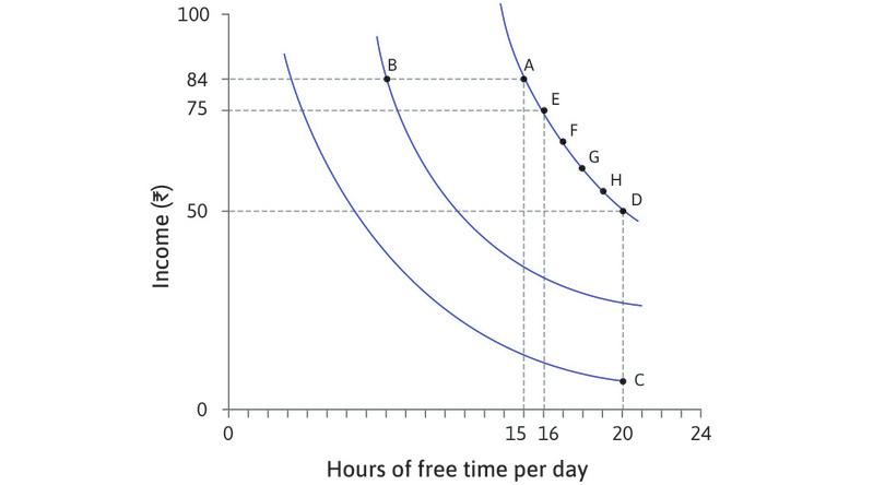
Figure 1 Mapping Sakina’s preferences.
The marginal rate of substitution
Given any combination \((t,\ y)\) of free time and income, Sakina’s marginal rate of substitution (MRS) (that is, her willingness to trade income for an extra hour of free time) is given by the slope of the indifference curve \(U(t,\ y)=c\) through that point.
How can we calculate the slope of the indifference curve \(U(t,\ y)=c\)?
To do this, we need to use the partial derivatives of the utility function. For example, \(\partial U/\partial t\) captures how utility changes as \((t)\) increases, holding \(y\) constant. In economics the partial derivative \(\partial U/\partial t\) is called the marginal utility of free time. Similarly \(\partial U/\partial y\) is the marginal utility of income. We have already noted that utility depends positively on \(t\) and \(y\). In other words, Sakina’s marginal utilities are both positive.
We calculate the slope of the indifference curve using a technique called implicit differentiation, which we shall meet again in later Leibnizes. In the present case, the method involves considering how cloth production would need to change if free time increased by a small amount, in order to keep utility constant.
Suppose both \(t\) and \(y\) change by small amounts \(\Delta t\) and \(\Delta y\). The small increments formula for functions of two variables gives an approximation to the change in utility \(\Delta U\), expressing it as the sum of a ‘free time effect’ and an ‘income effect’:
\[\Delta U \approx \frac{\partial U}{\partial t} \Delta t + \frac{\partial U}{\partial y} \Delta y\]If the changes \(\Delta t\) and \(\Delta y\) are such that Sakina stays on the same indifference curve, then her utility does not change; thus \(\Delta U = 0\), which implies that
\[\frac{\partial U}{\partial t} \Delta t + \frac{\partial U}{\partial y} \Delta y \approx 0\]Rearranging,
\[\frac{ \Delta y}{\Delta t} \approx - \frac{\partial U}{\partial t} \left/ \frac{\partial U}{\partial y} \right.\]The changes \(\Delta t\) and \(\Delta y\) together produce a small movement along an indifference curve. So if we now take the limit as \(\Delta t\to 0\), the left-hand side approaches the slope of that curve and the approximation becomes an equation.
Thus the slope of the indifference curve through any point \((t,\ y)\) is given by the formula:
\[\frac{dy}{dt} = -\frac{\partial U}{\partial t} \left/ \frac{\partial U}{\partial y} \right.\]- marginal rate of substitution (MRS)
- The trade-off that a person is willing to make between two goods. At any point, this is the slope of the indifference curve. See also: marginal rate of transformation.
The right-hand side of this equation is negative, since both marginal utilities are positive: increasing either free time or the income increases Sakina’s utility. Thus indifference curves slope downward, as in the diagram. To reduce confusion, we usually define the marginal rate of substitution (MRS) as the absolute value of the slope. So:
\[\text{MRS} = \left| \frac{\partial U}{\partial t} \left/ \frac{\partial U}{\partial y} \right. \right|\]or, in words,
\[\text{marginal rate of substitution} = \left| \frac{\text{marginal utility of free time}}{\text{marginal utility of income}} \right|\]Defining the MRS as a positive number allows us to say, for example, that the MRS is higher (Sakina is more willing to trade off income for free time) at points where the indifference curve is steeper, whereas the slope of the indifference curve is more negative at such points.
The MRS is the rate at which Sakina is prepared to trade income for additional hours of free time. The equation above, expressing the MRS as a ratio of marginal utilities, may be interpreted as follows: the MRS is approximately equal to the extra utility obtained from one more unit of free time, divided by the extra utility obtained from an additional rupee of income. As usual with interpretations of exact statements involving calculus in terms of individual units, the approximation is a good one if units are small quantities.
Convex preferences
Each indifference curve in Figure 1 becomes flatter as one moves along it to the right:
- marginal rate of substitution (MRS)
- The trade-off that a person is willing to make between two goods. At any point, this is the slope of the indifference curve. See also: marginal rate of transformation.
Sakina’s MRS falls if her free time becomes greater and her income decreases in such a way as to keep utility constant. This property of Sakina’s preferences is known as diminishing marginal rate of substitution and is usually assumed when we draw indifference curves with two goods.
Another way to describe this assumption is to note that Sakina’s indifference curves are convex. In algebraic terms, if we rewrite the equation of an indifference curve \(U(t,\ y)=c\) in the form \(y=g(t,\ c)\), then \(g(t,\ c)\) is a decreasing and convex function of \(t\) for given \(c\). We say that Sakina has convex preferences.
A person whose preferences are convex always prefers mixtures of goods to extremes of either good. If we draw a line between two points on the same indifference curve, then each point on the line is a mixture of the two end-points. When the indifference curves are convex, all points on the line between the end-points give higher utility than the end-points.
We shall give an example of a utility function displaying diminishing MRS in the next section.
Read more: Sections 14.2 (for the small increments formula) and 15.1 (for contours and implicit differentiation) of Malcolm Pemberton and Nicholas Rau. 2015. Mathematics for economists: An introductory textbook, 4th ed. Manchester: Manchester University Press.
An example: The Cobb-Douglas utility function
In this section, we look at a particular utility function that is often used in economic modelling. We derive expressions for the marginal utilities and the marginal rate of substitution, and verify their properties.
As before, Sakina cares about free time and her income. Suppose that her utility function is:
\[U (t,\ y)= t^\alpha y^\beta\]where \(\alpha\) and \(\beta\) are positive constants. This function has some very convenient mathematical properties. It is called a Cobb-Douglas function after the two people who introduced it into economics.
To find the marginal utilities of free time and income, we must find the partial derivatives of the utility function. Differentiating \(U\) with respect to \(t\), we see that the marginal utility of free time is:
\[\frac{\partial U}{\partial t} = \alpha t^{\alpha -1} y^\beta\]We know from the utility function that \(t^{\alpha -1} y^\beta = U/t\), which gives us a simpler expression for the marginal utility of free time:
\[\frac{\partial U}{\partial t} = \frac{\alpha U}{t}\]Similarly, the marginal utility of income is:
\[\frac{\partial U}{\partial y} = \beta t^{\alpha} y^{\beta-1} = \frac{\beta U}{y}\]Notice that when \(t\) and \(y\) are positive, so is \(U\). Hence the assumption that \(\alpha\) is also positive implies that \(\partial U/\partial t \gt0\). Similarly, \(\beta\gt0\) implies that \(\partial U/\partial y \gt0\). In other words, the assumption that both \(\alpha\) and \(\beta\) are positive ensures that ‘goods are good’: Sakina’s utility rises as free time or income increase.
In the previous section, we defined the marginal rate of substitution (MRS) between free time and income as the absolute value of the slope of an indifference curve, and showed that it was equal to the ratio of the marginal utility of free time to the marginal utility of the cloth production. With the Cobb-Douglas utility function:
\[\text{MRS} = \frac{\partial U}{\partial t} \left/ \frac{\partial U}{\partial y} \right. = \frac{\alpha U}{t} \left/ \frac{\beta U}{y} \right. = \frac{\alpha y}{\beta t}\]The indifference curves are downward sloping in \((t,\ y)\) space, so as we move to the right along an indifference curve, \(t\) rises and \(y\) falls, and thus \(y/t\) falls. Since \(\alpha\) and \(\beta\) are positive, MRS also falls. Thus, the Cobb-Douglas utility function implies diminishing MRS.
Read more: Sections 15.1 and 15.2 of Malcolm Pemberton and Nicholas Rau. 2015. Mathematics for economists: An introductory textbook, 4th ed. Manchester: Manchester University Press.
