3. Measuring the effect of a sugar tax Working in Python
Download the code
To download the code chunks used in this project, right-click on the download link and select ‘Save Link As…’. You’ll need to save the code download to your working directory, and open it in Python.
Don’t forget to also download the data into your working directory by following the steps in this project.
Python-specific learning objectives
In addition to the learning objectives for this project, in this section you will learn how to use method chaining to run a sequence of functions.
Getting started in Python
Head to the ‘Getting Started in Python’ page for help and advice on setting up a Python session to work with. Remember, you can run any page from this project as a notebook by downloading the relevant file from this repository and running it on your own computer. Alternatively, you can run pages online in your browser over at Binder.
Preliminary settings
Let’s import the packages we’ll need and also configure the settings we want:
import pandas as pd
import matplotlib as mpl
import matplotlib.pyplot as plt
import numpy as np
from pathlib import Path
import pingouin as pg
from lets_plot import *

LetsPlot.setup_html(no_js=True)
Part 3.1 Before-and-after comparisons of retail prices
We will first look at price data from the treatment group (stores in Berkeley) to see what happened to the price of sugary and non-sugary beverages after the tax.
- Download the ‘Berkeley Store Price Survey’ Excel dataset, which is taken from the Global Food Research Program’s website.
- The first tab of the Excel file contains the data dictionary. Make sure you read the data description column carefully, and check that each variable is in the Data tab.
Python walk-through 3.1 Importing the data file into Python
The data is stored in
.xlsxformat, so we use thepd.read_excelfunction from thepandaspackage to import it. We also import thematplotliblibrary as this includes packages that we will use later for drawing charts.If you open the data in Microsoft’s Excel, Apple’s Numbers, or LibreOffice’s Calc (free), you will see that there are two tabs: ‘Data Dictionary’, which contains some information about the variables, and ‘Data’, which contains the actual data. Let’s import both into Python, so that we don’t need to refer back to Excel for the additional information about variables.
Remember to store the downloaded file in a subdirectory of your current working directory called
data. Let’s import the data.path_to_data = Path("data/Dataset Project 3.xlsx") var_info = pd.read_excel(path_to_data, sheet_name="Data Dictionary") data = pd.read_excel(path_to_data, sheet_name="Data")Let’s use the
info()method to ensure that all the variables were given the correct datatypes:data.info()<class 'pandas.core.frame.DataFrame'> RangeIndex: 2175 entries, 0 to 2174 Data columns (total 12 columns): # Column Non-Null Count Dtype --- ------ -------------- ----- 0 store_id 2175 non-null int64 1 type 2175 non-null object 2 store_type 2175 non-null int64 3 type2 235 non-null object 4 size 2175 non-null float64 5 price 2175 non-null float64 6 price_per_oz 2175 non-null float64 7 price_per_oz_c 2175 non-null float64 8 taxed 2175 non-null int64 9 supp 2175 non-null int64 10 time 2175 non-null object 11 product_id 2175 non-null int64 dtypes: float64(4), int64(5), object(3) memory usage: 204.0+ KBPython classified all the variables containing numbers as either
int64(integers) orfloat64(real numbers). However, other variables were labelled asobjectbecause they don’t contain numbers, and some of the columns labelled as numbers are actually categorical variables (there are a fixed number of categories).In the next section, we’re going to use a ‘for’ loop. This loop has the syntax:
for thing in things, then a colon (:), then an indented expression that does some operation onthing.We are using a ‘for’ loop to redefine a list of incorrectly defined variables (such as
taxed) as categorical data types. Rather than laboriously run the same code multiple times (data["type"] = data["type"].astype("category")and thendata["taxed"] = data["taxed"].astype("category"), and so on), we can just have a list of variables we’d like to convert and then use a ‘for’ loop to apply the same kind of command to each variable. In the code below,colis our ‘thing’ (according to the ‘for’ loop syntax). When Python gets todata[col] = data[col].astype("category")it will replacecolwith each element in the list of things we feed it in turn.So now let’s ensure that
type,taxed,supp,store_id,store_type,type2andproduct_idare represented as categorical variables. We’ll use theastypefunction to convert them within a ‘for’ loop.for col in ["type", "taxed", "supp", "store_id", "store_type", "type2", "product_id"]: data[col] = data[col].astype("category") # rename some of the categories data["taxed"] = data["taxed"].cat.rename_categories(["not taxed", "taxed"]) data["supp"] = data["supp"].cat.rename_categories(["standard", "supplemental"]) data["store_type"] = data["store_type"].cat.rename_categories( ["Large supermarket", "Small supermarket", "Pharmacy", "Gas station"] )You can see that we used
.cat.rename_categoriesto give more meaningful names to different categories (where they are clearly defined).There is another variable,
time, which is classified as having anobjectdatatype, but should be a categorical variable. Before we do this, we use theuniquecommand to check the categories of this variable.data["time"].unique()array(['DEC2014', 'JUN2015', 'MAR2015'], dtype=object)If you look at the timeline in the Silver et al. (2017) paper, you will notice that the third price survey was in March 2016, not in March 2015, so the data has been labelled incorrectly. We shall therefore change all the values
MAR2015toMAR2016.data.loc[data["time"] == "MAR2015", "time"] = "MAR2016"We can now change
timeinto a categorical variable.data["time"] = data["time"].astype("category")
- Read ‘S1 Text’, from the journal paper’s supporting information, which explains how the Store Price Survey data was collected.
- In your own words, explain how the product information was recorded, and the measures that researchers took to ensure that the data was accurate and representative of the treatment group. What were some of the data collection issues that they encountered?
- Instead of using the name of the store, each store was given a unique ID number (recorded as
store_idon the spreadsheet). Verify that the number of stores in the dataset is the same as that stated in the ‘S1 Text’ (26). Similarly, each product was given a unique ID number (product_id). How many different products are in the dataset?
Python walk-through 3.2 Counting the number of unique elements in a variable
We use two methods here: the
uniquefunction to obtain a list of the unique elements of the variables of interest (data["store_id"]anddata["product_id"]), thenlento count how long the list is. We will create two variables,no_storesandno_products, that contain the number of stores and products respectively.no_stores = len(data["store_id"].unique()) no_products = len(data["product_id"].unique()) print(f"The {no_stores=} while the {no_products=}.")The no_stores=26 while the no_products=247.
Following the approach described in ‘S1 Text’, we will compare the variable price per ounce in US$ cents (price_per_oz_c). We will look at what happened to prices in the two treatment groups before the tax (time = DEC2014) and after the tax (time = JUN2015):
- treatment group one: large supermarkets (
store_type = 1) - treatment group two: pharmacies (
store_type = 3).
Before doing this analysis, we will use summary measures to see how many observations are in the treatment and control group, and how the two groups differ across some variables of interest. For example, if there are very few observations in a group, we might be concerned about the precision of our estimates and will need to interpret our results in light of this fact.
We will now create frequency tables containing the summary measures that we are interested in.
- Create the following tables:
- A frequency table showing the number (count) of store observations (store type) in December 2014 and June 2015, with
store_typeas the row variable andtime_periodas the column variable. For each store type, is the number of observations similar in each time period?
- A frequency table showing the number of taxed and non-taxed beverages in December 2014 and June 2015, with
store_typeas the row variable andtaxedas the column variable. (Taxedequals 1 if the sugar tax applied to that product, and 0 if the tax did not apply). For each store type, is the number of taxed and non-taxed beverages similar?
- A frequency table showing the number of each product type (type), with
product_typeas the row variable andtime_periodas the column variable. Which product types have the highest number of observations and which have the lowest number of observations? Why might some products have more observations than others?
Python walk-through 3.3 Creating frequency tables
Frequency table for store type and time period
We use the
pd.crosstabfunction to perform a cross-tabulation count ofstore_typebytime.pd.crosstab(index=data["store_type"], columns=data["time"])
time DEC2014 JUN2015 MAR2016 store_type Large supermarket 177 209 158 Small supermarket 407 391 327 Pharmacy 87 102 73 Gas station 73 96 75 There are fewer observations taken from gas stations and pharmacies and more from small supermarkets.
Frequency table for store type and taxed
Now we repeat the steps above to make a frequency table with
store_typeas the row variable andtaxedas the column variable. We pass a list of dataframe columns to thepd.crosstabfunction because we also want separate values for each time period. To get the total row each row and column, we addmargins=True.pd.crosstab( index=data["store_type"], columns=[data["time"], data["taxed"]], margins=True )
time DEC2014 JUN2015 MAR2016 All taxed not taxed taxed not taxed taxed not taxed taxed not taxed store_type Large supermarket 92 85 111 98 88 70 544 Small supermarket 196 211 192 199 154 173 1125 Pharmacy 44 43 52 50 36 37 262 Gas station 34 39 44 52 31 44 244 All 366 378 399 399 309 324 2175 Frequency table for product type and time period
Now we make a frequency table with product type (
type) as the row variable and time period (time) as the column variable.pd.crosstab(index=data["type"], columns=data["time"], margins=True)
time DEC2014 JUN2015 MAR2016 All type ENERGY 56 58 49 163 ENERGY-DIET 49 54 35 138 JUICE 70 64 52 186 JUICE DRINK 19 17 6 42 MILK 63 61 53 177 SODA 239 262 215 716 SODA-DIET 128 174 127 429 SPORT 11 16 12 39 SPORT-DIET 2 2 0 4 TEA 52 45 41 138 TEA-DIET 6 6 8 20 WATER 48 38 34 120 WATER-SWEET 1 1 1 3 All 744 798 633 2175 This table shows that there were no observations for the category
SPORT–DIETin March 2016. As this is a drink which even in the other months has very few observations, it may be a product that is offered only in one shop, and it is possible that this shop was not visited in March 2016. The product may also be a seasonal product that is not available in March. It is also likely thatWATER–SWEETis offered in only one shop.
- conditional mean
- An average of a variable, taken over a subgroup of observations that satisfy certain conditions, rather than all observations.
Besides counting the number of observations in a particular group, we can also calculate the mean by only using observations that satisfy certain conditions (known as the conditional mean). In this case, we are interested in comparing the mean price of taxed and untaxed beverages, before and after the tax.
- Calculate and compare conditional means:
- Create a table similar to Figure 3.1, showing the average price per ounce (in cents) for taxed and untaxed beverages separately, with
store_typeas the row variable, andtaxedandtimeas the column variables. To follow the methodology used in the journal paper, make sure to only include products that are present in all time periods, and non-supplementary products (supp = 0).
- Without doing any calculations, summarize any differences or general patterns between December 2014 and June 2015 that you find in the table.
- Would we be able to assess the effect of sugar taxes on product prices by comparing the average price of untaxed goods with that of taxed goods in any given period? Why or why not?
| Non-taxed | Taxed | |||
|---|---|---|---|---|
| Store type | Dec 2014 | Jun 2015 | Dec 2014 | Jun 2015 |
| 1 | ||||
| 3 | ||||
Figure 3.1 The average price of taxed and non-taxed beverages, according to time period and store type.
Python walk-through 3.4 Calculating conditional means
Calculating conditional, or group, means is a common data cleaning operation you will encounter. It can be a bit confusing, but, in the typical case, we might just be asking what the mean is for each period (instead of the mean for all periods). Also, we must choose whether to put the mean back into our data with the original index (and so the original number of rows) or with a new index that reflects what the mean is conditional on. We’ll now see one way to do this.
In order to identify products (
product_id) that have observations for all three periods (DEC2014,JUN2015andMAR2016), we will first create a new variable calledperiod_test, which takes the valueTrueif we have observations in all periods for a product in a particular store, andFalseotherwise. These true/false variables are called Boolean variables.This is going to be a complex operation with several steps. First, we’ll use a
groupbyoperation to group everything byproduct_idandstore_id. Then we’ll select the column we want (time). Then we’ll usetransform: this command returns a series with the same number of rows as the original index, so will fit nicely into our existing dataframe (rather than having the index set as the number of unique groups from thegroupbyoperation). Within ourtransform, we’ll ask for the number of unique (nunique) categories of time. For entries that exist, this value will be 1, 2, or 3 depending on whether the product is available in 1, 2, or 3 of the periods. For entries that don’t exist, this value will beNaN, which means ‘not a number’. So we then use.fillna(0)to set these to zero. Finally we compare this object against the known unique number of different periods (3) to get ourTrueorFalsevalue; in this case,Trueif there are 3 periods, andFalseotherwise.data.groupby(["product_id", "store_id"])["time"].transform( lambda x: x.nunique() ).fillna(0) == data["time"].nunique()0 True 1 False 2 False 3 True 4 False ... 2170 True 2171 True 2172 True 2173 True 2174 True Name: time, Length: 2175, dtype: boolTip: The
pandasdocumentation provides many detailed examples of its extensive functionality, including thetransformfunction.Let’s store this in the dataframe as a new column called
period_test:data["period_test"] = ( data.groupby(["product_id", "store_id"])["time"] .transform(lambda x: x.nunique()) .fillna(0) == data["time"].nunique() )Now we can check this code worked by picking out the first unique
product_id,store_idcombination:data.loc[(data["product_id"] == 29) & (data["store_id"] == 16), :]
store_id type store_type type2 size price price_per_oz price_per_oz_c taxed supp time product_id period_test 0 16 WATER Small supermarket NaN 33.8 1.69 0.050000 5.000000 not taxed standard DEC2014 29 True 744 16 WATER Small supermarket NaN 33.8 1.79 0.052959 5.295858 not taxed standard JUN2015 29 True 1542 16 WATER Small supermarket NaN 33.8 1.69 0.050000 5.000000 not taxed standard MAR2016 29 True
period_testreportsTruefor this combination, and we can see that all three periods are present. Let’s try anotherproduct_id,store_idcombination:data.loc[(data["product_id"] == 29) & (data["store_id"] == 10), :]
store_id type store_type type2 size price price_per_oz price_per_oz_c taxed supp time product_id period_test 69 10 WATER Small supermarket NaN 33.8 1.75 0.051775 5.177515 not taxed standard DEC2014 29 False 817 10 WATER Small supermarket NaN 33.8 1.99 0.058876 5.887574 not taxed standard JUN2015 29 False In this case, the product-store cell is only there for two out of the three periods and so gets a
Falseentry for itsperiod_testcolumn.Now we can use the
period_testvariable to remove all products that have not been observed in all three periods. We’ll also filter bystandardin the"supp"column. We will store the remaining products in a new dataframe,data_c.data_c = data.loc[data["period_test"] & (data["supp"] == "standard")] data_c.head()
store_id type store_type type2 size price price_per_oz price_per_oz_c taxed supp time product_id period_test 0 16 WATER Small supermarket NaN 33.8 1.69 0.050000 5.000000 not taxed standard DEC2014 29 True 3 16 WATER Small supermarket NaN 33.8 1.69 0.050000 5.000000 not taxed standard DEC2014 38 True 5 16 MILK Small supermarket LOW FAT MILK 64.0 2.79 0.043594 4.359375 not taxed standard DEC2014 41 True 7 16 MILK Small supermarket WHOLE MILK 64.0 2.79 0.043594 4.359375 not taxed standard DEC2014 43 True 10 16 SODA Small supermarket NaN 20.0 1.89 0.094500 9.450000 taxed standard DEC2014 59 True Now we can calculate the means of
price_per_ozby grouping the data according tostore_type,taxed, andtime.You may have noticed that we’re stringing together multiple methods, with one called after another like
.method1(options).method2(options). This is a technique called method chaining: it just means chaining many successive methods together one after another.Method chaining is a useful technique for data analysis, but it has advantages and disadvantages. If you know what the code is doing, and that it works already, it can be substantially easier to read than successive lines of logic using assignment via
=. However, if something is going wrong within a long method chain, it can be hard to know where and why.You can find a deeper dive into method chaining in the relevant section of Coding for Economists.
In the code below, we’re going to use a lot of method chaining to get the data we want. The first operation in the chain groups all of the variables together by
taxed,store_type, andtime. The second operation produces some new columns via.agg. The column names,avg_priceandn, are specified via the("input column", "function to be applied")syntax. The new dataframe has thegroupbyvariables as its index, so we reset the index to row numbers (.reset_index). We can then perform apivotto transform the data into the shape that we want.One point to note is that the
new_column_name = ("input column", "function to be applied")syntax is special topandas, so you likely won’t see it in other packages. However, it is quite convenient in this case where we have quite a few bespoke operations and new column names being introduced all at once—and it’s really helpful for method chaining!table_res = ( data_c.groupby(["taxed", "store_type", "time"]) .agg(avg_price=("price_per_oz", "mean"), n=("price_per_oz", "count")) .reset_index() .pivot(index=["taxed", "store_type", "n"], columns="time", values="avg_price") ) table_res
time DEC2014 JUN2015 MAR2016 taxed store_type n not taxed Large supermarket 36 0.111920 0.114804 0.117015 Small supermarket 70 0.136708 0.138165 0.133672 Pharmacy 18 0.151958 0.160754 0.154353 Gas station 12 0.169351 0.169641 0.170414 taxed Large supermarket 36 0.156174 0.169297 0.166843 Small supermarket 101 0.158510 0.159952 0.154925 Pharmacy 18 0.181818 0.190788 0.186303 Gas station 22 0.194117 0.203367 0.192376 Use the S3 Table in the journal paper to check how closely your summary data match those in the paper. You should find that your results for Large Supermarkets and Pharmacies match, but the other store types have discrepancies. In Python walk-through 3.5, we will discuss these differences in more detail.
In order to make a before-and-after comparison, we will make a chart similar to Figure 2 in the journal paper, to show the change in prices for each store type.
- Using your table from Question 3:
- Calculate the change in the mean price after the tax (price in June 2015 minus price in December 2014) for taxed and untaxed beverages, by store type.
- Using the values you calculated in Question 4(a), plot a column chart to show this information (as done in Figure 2 of the journal paper) with store type on the horizontal axis and price change on the vertical axis. Label each axis and data series appropriately. You should get the same values as shown in Figure 2.
Python walk-through 3.5 Making a column chart to compare two groups
Calculate price differences by store type
Let’s calculate the two price differences (June 2015 minus December 2014 and March 2016 minus December 2014), and store them as
d1andd2, respectively:table_res["d1"] = table_res["JUN2015"] - table_res["DEC2014"] table_res["d2"] = table_res["MAR2016"] - table_res["DEC2014"] table_res
time DEC2014 JUN2015 MAR2016 d1 d2 taxed store_type n not taxed Large supermarket 36 0.111920 0.114804 0.117015 0.002884 0.005096 Small supermarket 70 0.136708 0.138165 0.133672 0.001458 −0.003036 Pharmacy 18 0.151958 0.160754 0.154353 0.008796 0.002395 Gas station 12 0.169351 0.169641 0.170414 0.000290 0.001063 taxed Large supermarket 36 0.156174 0.169297 0.166843 0.013122 0.010669 Small supermarket 101 0.158510 0.159952 0.154925 0.001442 −0.003585 Pharmacy 18 0.181818 0.190788 0.186303 0.008970 0.004485 Gas station 22 0.194117 0.203367 0.192376 0.009251 −0.001740 Plot a column chart for average price changes
To display
d1andd2in a column chart, we will use thegeom_barfunction in thelets_plotpackage, which we loaded at the start of this project. We’ll usestat="identity"to getlets_plotto use the numbers in the dataframe rather than the count of entries in the dataframe (which is its default).position_dodge()causes the two types we are looking at in"taxed"to appear side-by-side rather than overlaid.Let’s start with displaying the average price change from December 2014 to June 2015 (which is stored in
d1).( ggplot(table_res.reset_index(), aes(fill="taxed", y="d1", x="store_type")) + geom_bar(stat="identity", position=position_dodge()) + labs( y="Price change (US$/oz)", x="Store type", title="Average price change from Dec 2014 to Jun 2015", fill="Beverages", ) )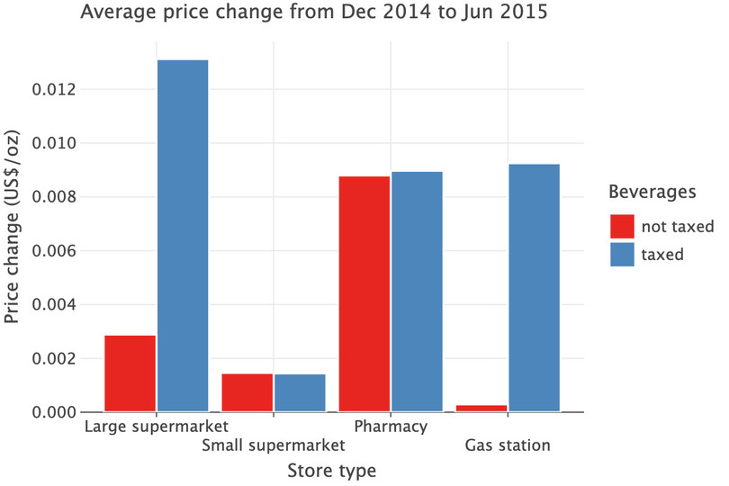
![Average price change from December 2014 to June 2015.]()
Figure 3.2 Average price change from December 2014 to June 2015.
Now we do the same for the price change from Dec 2014 to Mar 2016:
(
    ggplot(table_res.reset_index(), aes(fill="taxed", y="d2", x="store_type"))
    + geom_bar(stat="identity", position=position_dodge())
    + labs(
        y="Price change (US$/oz)",
        x="Store type",
        title="Average price change from Dec 2014 to Mar 2016",
        fill="Beverages",
    )
)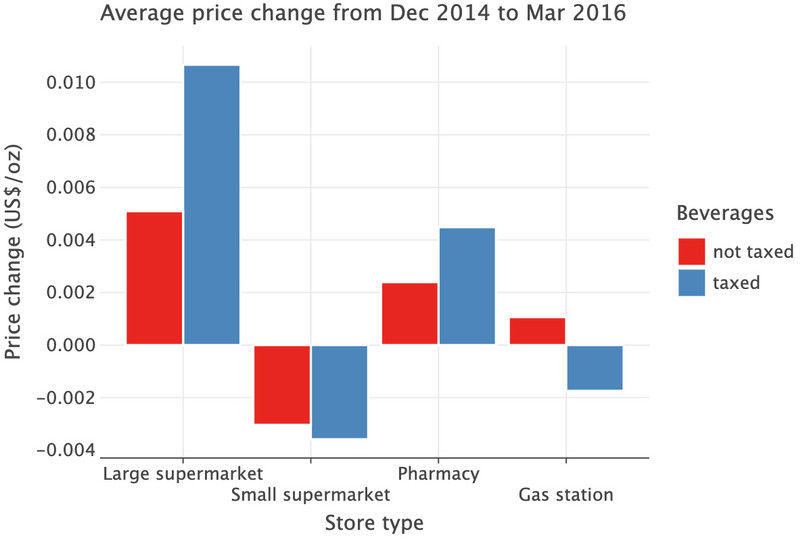
![Average price change from December 2014 to Marrch 2016.]()
Figure 3.3 Average price change from December 2014 to March 2016.
- statistically significant
- When a relationship between two or more variables is unlikely to be due to chance, given the assumptions made about the variables (for example, having the same mean). Statistical significance does not tell us whether there is a causal link between the variables.
To assess whether the difference in mean prices before and after the tax could have happened by chance due to the samples chosen (and there are no differences in the population means), we could calculate the p-value. (Here, ‘population means’ refer to the mean prices before/after the tax that we would calculate if we had all prices for all stores in Berkeley.) The authors of the journal article calculate p-values, and use the idea of statistical significance to interpret them. Whenever they get a p-value of less than 5%, they conclude that the assumption of no differences in the population is unlikely to be true: they say that the price difference is statistically significant. If they get a p-value higher than 5%, they say that the difference is not statistically significant, meaning that they think it could be due to chance variation in prices.
Using a particular cutoff level for the p-value, and concluding that a result is only statistically significant if the p-value is below the cutoff, is common in statistical studies, and 5% is often used as the cutoff level. But this approach has been criticized recently by statisticians and social scientists. The main criticisms raised are that any cutoffs are arbitrary. Instead of using a cutoff, we prefer to calculate p-values and use them to assess the strength of the evidence against our assumption that there are no differences in the population means. Whether the statistical evidence is strong enough for us to draw a conclusion about a policy, such as a sugar tax, will always be a matter of judgement.
According to the journal paper, the p-value is 0.02 for large supermarkets, and 0.99 for pharmacies.
- Based on these p-values and your chart from Question 4, what can you conclude about the difference in means? (Hint: You may find the discussion in Part 2.3 helpful.)
Extension Python walk-through 3.6 Calculating the p-value for price changes
In this walk-through, we show the calculations required to obtain the p-values in Table S3 of the Silver et al. (2017) paper. Since the p-values are already provided, this walk-through is only for those who want to see how these p-values were calculated. For the categories of Large supermarkets and Pharmacies, we conduct a hypothesis test, which tests the null hypothesis that the price difference between June 2015 and December 2014 (and March 2016 and December 2014) for the taxed and untaxed beverages in the two store types could be due to chance.
We are interested in whether the difference in average price between
JUN2015andDEC2014(orMAR2016andDEC2014) for one group (say, Large supermarket and taxed beverages) is zero (i.e. there is no difference in the means of the two populations). Note that we are dealing with paired observations (the same product in both time periods).Let’s use the price difference between June 2015 and December 2014 in Large supermarkets for taxed beverages as an example. First, we extract the prices for both periods (the vectors
p_1andp_2) and then calculate the difference, element by element (stored asd_t). Because all operations assume the same index, we must also reset the indexes of these sets of values that have been drawn from different rows (dropping the original indexes as we go).In the code below, we’re going to use a different way to cut a dataframe:
query. Previously, to filter down a dataframe by the values in its columns, we’ve used.locwith the filters we wanted. For example, to filter rows withvalue_aincolumn1andvalue_bincolumn2:df.loc[(df[column1] == "value_a") & (df[column2]=="value_b"), :]This syntax can result in very long lines of code.
queryallows you to write something that is shorter and is composed of a single string (which sometimes comes in handy). The syntax forqueryusescol_name == 'value_name'with&to join multiple filters together. Note that if the value used to filter the column is numeric instead of string or category, you do not need the inner quotes, for example,col_name = 85.p_1 = data_c.query( "store_type == 'Large supermarket' & taxed == 'taxed' & time == 'DEC2014'" )["price_per_oz"].reset_index(drop=True) p_2 = data_c.query( "store_type == 'Large supermarket' & taxed == 'taxed' & time == 'JUN2015'" )["price_per_oz"].reset_index(drop=True) # Price difference for taxed products in large supermarkets d_t = p_2 - p_1 d_t.head()0 0.010000 1 0.010059 2 0.009600 3 0.010000 4 0.010059 Name: price_per_oz, dtype: float64All three new variables are vectors with 36 elements. For
d_tto correctly represent the price difference for a particular product in a particular store, we need to be certain that each element in both vectors corresponds to the same product in the same store.To check that the elements match, we will extract the store and product IDs along with the prices, and save it as
alt. We will then compare the ordering in theDEC2014column (p1_alt) and theJUN2015column (p2_alt).alt = data_c.loc[ (data_c["store_type"] == "Large supermarket") & (data_c["taxed"] == "taxed"), : ].pivot(index=["store_id", "product_id"], columns="time", values="price_per_oz") alt.head()
time DEC2014 JUN2015 MAR2016 store_id product_id 25 59 0.099500 0.109500 0.109500 60 0.032396 0.042456 0.042456 153 0.135200 0.144800 0.144800 189 0.094500 0.104500 0.109500 190 0.029438 0.039497 0.039497 Now we can simply subtract column
p_2_altfromp_1_alt, preserving the index. We’ll save this difference asd_t_alt.p_1_alt, p_2_alt = alt["DEC2014"], alt["JUN2015"] d_t_alt = p_2_alt - p_1_alt d_t_alt.head()store_id product_id 25 59 0.010000 60 0.010059 153 0.009600 189 0.010000 190 0.010059 dtype: float64Note that in this case, we can also see which combination produced this particular value of the
price_per_oz. This approach guarantees identical ordering because the subtraction would fail if the indices were different.The average value of the price difference is 0.1312, and our task is to evaluate whether this is likely to be due to sampling variation (given the assumption that there is no difference between the populations) or not. To do this, we can use the
ttestfunction, which provides the associated p-value.# Recognise that the differences come from paired samples. pg.ttest(p_2, p_1, paired=True)
T dof alternative p-val CI95% cohen-d BF10 power ttest 4.768132 35 two-sided 0.000032 [0.01, 0.02] 0.079958 699.454 0.075305 Alternatively, we can calculate the respective test statistic manually, which also requires us to calculate the standard error of this value:
d_t_alt.mean() / np.sqrt((d_t_alt.var() / len(d_t_alt)))4.768131783937789Yet another alternative is to use the
ttestfunction directly ond_t.To compare this result to the journal paper, look at the extract from Table S3 (the section on Large supermarkets) shown in Figure 3.4 below. The cell with
**shows the mean price difference of 1.31 cents ($0.0131).
Large supermarkets
(n = 6)Taxed beverage price
(36 sets)Untaxed beverage price
(36 sets)Taxed – untaxed difference cents/oz cents/oz cents/oz Round 1: December 2014 15.62 11.19 Round 2: June 2015 16.93 11.48 Round 3: March 2016 16.68 11.70 Mean change
(March 2016–Dec 2014)1.07, (p=0.01) 0.51, (p=0.01) 0.56, (p=0.22) Mean change
(June 2015–Dec 2014)1.31, (p<0.001)** 0.29, (p=0.08) 1.02, (p=0.002) Figure 3.4 Table S3 in Silver et al. (2017), showing means and confidence intervals. n = number of stores of each type.
In our test output, we get a very small p-value (0.000032) which in the table is indicated by the double asterisk.
Tests for other store types are calculated similarly, by changing the data extracted to
p_1andp_2. Let’s do that for one more example: the price difference between June 2015 and December 2014 in Large supermarkets for untaxed beverages.alt_nt = data_c.loc[ (data_c["store_type"] == "Large supermarket") & (data_c["taxed"] == "not taxed"), : ].pivot(index=["store_id", "product_id"], columns="time", values="price_per_oz") d_nt_alt = alt_nt["JUN2015"] - alt_nt["DEC2014"] print(f"Mean difference is {100*Δ_nt_alt.mean():.2f} cents/oz") pg.ttest(d_nt_alt, y=0)Mean difference is 0.29 cents/oz
T dof alternative p-val CI95% cohen-d BF10 power ttest 1.817855 35 two-sided 0.077655 [−0.0, 0.01] 0.302976 0.788 0.423962 You should be able to recognise the mean difference and the p-value in the excerpt of Table S3 provided in Figure 3.4.
Let’s also replicate the last section of Table S3, which shows the difference between the price changes in taxed and untaxed products, that is, we want to know whether
d_t_altandd_nt_althave different means. We will apply the two sample hypothesis tests, but this time for unpaired data, as the products differ across samples.pg.ttest(d_t_alt, d_nt_alt)
T dof alternative p-val CI95% cohen-d BF10 power ttest 3.222715 70 two-sided 0.001929 [0.0, 0.02] 0.759601 17.601 0.888432 Again you should be able to identify the corresponding entries in Table S3 shown in Figure 3.4. The main entry in the table is 1.02, indicating that the means of the two groups differ by 1.02 cents. This is confirmed in our calculations, as $0.01312 − $0.00288 is about $0.0102 or 1.02 cents. The p-value of 0.002 is also the same as the one in Table S3.
Part 3.2 Before-and-after comparisons with prices in other areas
When looking for any price patterns, it is possible that the observed changes in Berkeley were not solely due to the tax, but instead were also influenced by other events that happened in Berkeley and in neighbouring areas. To investigate whether this is the case, the researchers conducted another differences-in-differences analysis, using a different treatment and control group:
- The treatment group: Beverages in Berkeley
- The control group: Beverages in surrounding areas.
The researchers collected price data from stores in the surrounding areas and compared them with prices in Berkeley. If prices changed in a similar way in nearby areas (which were not subject to the tax), then what we observed in Berkeley may not be primarily a result of the tax. We will be using the data the researchers collected to make our own comparisons.
Download the following files:
- The Berkeley Point-of-Sale Stata file on the Global Food Research Program’s website, containing the price data they collected, including information on the date (year and month), location (Berkeley or non-Berkeley), beverage group (soda, fruit drinks, milk substitutes, milk and water), and the average price for that month. Stata is another popular statistical software package, and the data is provided as a
.dtafile. - ‘S5 Table’ which compares the neighbourhood characteristics of the Berkeley and non-Berkeley stores.
- Based on ‘S5 Table’, do you think the researchers chose suitable comparison stores? Why or why not?
We will now plot a line chart similar to Figure 3 in the journal paper, to compare prices of similar goods in different locations and see how they have changed over time. To do this, we will need to summarize the data so that there is one value (the mean price) for each location and type of good in each month.
- Assess the effects of a tax on prices:
- Create a table similar to the one provided in Figure 3.5 to show the average price in each month for taxed and non-taxed beverages, according to location. Use ‘year and month’ as the row variables, and ‘tax’ and ‘location’ as the column variables. (Hint: You may find Python walk-through 3.4 helpful.)
- Plot the four columns of your table on the same line chart, with average price on the vertical axis and time (months) on the horizontal axis. Describe any differences you see between the prices of non-taxed goods in Berkeley and those outside Berkeley, both before the tax (January 2013 to December 2014) and after the tax (March 2015 onwards). Do the same for prices of taxed goods.
- Based on your chart, is it reasonable to conclude that the sugar tax had an effect on prices?
| Non-taxed | Taxed | |||
|---|---|---|---|---|
| Year/Month | Berkeley | Non-Berkeley | Berkeley | Non-Berkeley |
| January 2013 | ||||
| February 2013 | ||||
| March 2013 | ||||
| … | ||||
| December 2013 | ||||
| January 2014 | ||||
| … | ||||
| February 2016 | ||||
Figure 3.5 The average price of taxed and non-taxed beverages, according to location and month.
Python walk-through 3.7 Importing data from a Stata file and plotting a line chart
Import data and create a table of average monthly prices
To import data from a Stata file (
.dtaformat) we need thepandaspackage’spd.read_statafunction. Remember to download the data from this link and save the file with extension.dtain thedata/folder of your working directory.path_to_stata_data = Path("data/public_use_weighted_prices2.dta") posd = pd.read_stata(path_to_stata_data) posd.head()
year quarter month location beverage_group tax price under_report 0 2013.0 1.0 1.0 Berkeley soda Non-taxed 4.853399 NaN 1 2013.0 1.0 1.0 Non-Berkeley soda Non-taxed 3.510271 NaN 2 2013.0 1.0 1.0 Non-Berkeley soda Non-taxed 3.889572 NaN 3 2013.0 1.0 1.0 Berkeley soda Taxed 3.682805 NaN 4 2013.0 1.0 1.0 Non-Berkeley soda Taxed 3.516437 NaN For each month and location (Berkeley or Non-Berkeley), there are prices for a variety of beverage categories, and we know whether the category is taxed or not. For any particular time-location-tax status combination, we want the average price of all products.
To make the summary table, we use method chaining again:
table_test = (
    posd.groupby(["year", "month", "location", "tax"])["price"]
    .agg("mean")
    .reset_index()
)
table_test
year month location tax price 0 2013.0 1.0 Berkeley Non-taxed 5.722480 1 2013.0 1.0 Berkeley Taxed 8.692803 2 2013.0 1.0 Non-Berkeley Non-taxed 5.348640 3 2013.0 1.0 Non-Berkeley Taxed 7.991574 4 2013.0 2.0 Berkeley Non-taxed 5.806468 ... ... ... ... ... ... 151 2016.0 2.0 Non-Berkeley Taxed 8.729508 152 2016.0 3.0 Berkeley Non-taxed NaN 153 2016.0 3.0 Berkeley Taxed NaN 154 2016.0 3.0 Non-Berkeley Non-taxed NaN 155 2016.0 3.0 Non-Berkeley Taxed NaN We’ll now prepare the data for plotting in a line chart.
First, we reset the index so that it is just composed of row numbers. We’d also like to add a column for time, recorded as a time series (in this case, a sequence of years and months).
table_test["date"] = (
    table_test.apply(
        lambda row: pd.to_datetime(
            str(int(row["year"])) + "-" + str(int(row["month"])), format="%Y-%m"
        ),
        axis=1,
    )
    + pd.offsets.MonthEnd()
)
table_test.head()
year month location tax price date 0 2013.0 1.0 Berkeley Non-taxed 5.722480 2013-01-31 1 2013.0 1.0 Berkeley Taxed 8.692803 2013-01-31 2 2013.0 1.0 Non-Berkeley Non-taxed 5.348640 2013-01-31 3 2013.0 1.0 Non-Berkeley Taxed 7.991574 2013-01-31 4 2013.0 2.0 Berkeley Non-taxed 5.806468 2013-02-28 Here, we create a variable called
dateby passing an integer version of the year and month together as a string topd.to_datetime, specifying the date format as YYYY-MM format (%Y-%m). This code produces a date at the start of each month;pd.offsets.MonthEnd()finds the last day in the month.In the code above, we used
applyandlambdaagain, both methods that we’ve seen before. Remember that, given an axis (axis=), the apply method applies a function to every element. Here we apply it to every row (axis=1) because the date column we want to create relies on combining information from different columns for each row.Plot a line chart
Now we can create a line chart.
date_one = pd.to_datetime("2015-01-01")
date_two = pd.to_datetime("2015-03-01")

# Rename 'date' as 'Date' for the horizontal axis label
table_test = table_test.rename(columns={'date': 'Date'})
(
    ggplot(table_test, aes(x="Date", y="price", color="tax", linetype="location"))
    + geom_vline(xintercept=date_one, color="gray")
    + geom_vline(xintercept=date_two, color="gray")
    + geom_line(size=1)
    + geom_text(
        x=date_one - pd.DateOffset(months=3), y=5, label="Pre-tax", color="black"
    )
    + geom_text(
        x=date_two + pd.DateOffset(months=3), y=5, label="Post-tax", color="black"
    )
    + labs(y="Price", color="Tax", linetype="Location")
)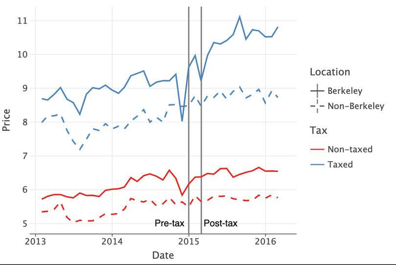
![Average price of taxed and non-taxed beverages in Berkeley and non-Berkeley areas.]()
Figure 3.6 Average price of taxed and non-taxed beverages in Berkeley and non-Berkeley areas.
How strong is the evidence that the sugar tax affected prices? According to the journal paper, when comparing the mean Berkeley and non-Berkeley price of sugary beverages after the tax, the p-value is smaller than 0.00001, and it is 0.63 for non-sugary beverages after the tax.
- What do the p-values tell us about the difference in means and the effect of the sugar tax on the price of sugary beverages? (Hint: You may find the discussion in Part 2.3 helpful.)
The aim of the sugar tax was to decrease consumption of sugary beverages. Figure 3.7 shows the mean number of calories consumed and the mean volume consumed before and after the tax. The researchers reported the p-values for the difference in means before and after the tax in the last column.
| Usual intake | Pre-tax (Nov–Dec 2014), n = 623 |
Post-tax (Nov–Dec 2015), n = 613 |
Pre-tax–post-tax difference | ||
|---|---|---|---|---|---|
| Caloric intake (kilocalories/capita/day) | |||||
| Taxed beverages | 45.1 | 38.7 | −6.4, p = 0.56 | ||
| Non-taxed beverages | 115.7 | 147.6 | 31.9, p = 0.04 | ||
| Volume of intake (grams/capita/day) | |||||
| Taxed beverages | 121.0 | 97.0 | −24.0, p = 0.24 | ||
| Non-taxed beverages | 1,839.4 | 1,896.5 | 57.1, p = 0.22 | ||
| Models account for age, gender, race/ethnicity, income level, and educational attainment. n is the sample size at each round of the survey after excluding participants with missing values on self-reported race/ethnicity, age, education, income, or monthly intake of sugar-sweetened beverages. | |||||
Figure 3.7 Changes in prices, sales, consumer spending, and beverage consumption one year after a tax on sugar-sweetened beverages in Berkeley, California, US: A before-and-after study.
Lynn D. Silver, Shu Wen Ng, Suzanne Ryan-Ibarra, Lindsey Smith Taillie, Marta Induni, Donna R. Miles, Jennifer M. Poti, and Barry M. Popkin. 2017. Table 1 in ‘Changes in prices, sales, consumer spending, and beverage consumption one year after a tax on sugar-sweetened beverages in Berkeley, California, US: A before-and-after study’. PLoS Med 14 (4): e1002283.
- Based on Figure 3.7, what can you say about consumption behaviour in Berkeley after the tax? Suggest some explanations for the evidence.
- Read the ‘Limitations’ in the ‘Discussions’ section of the paper and discuss the strengths and limitations of this study. How could future studies on the sugar tax in Berkeley address these problems? (Some issues you may want to discuss are: the number of stores observed, number of people surveyed, and the reliability of the price data collected.)
- Suppose that you have the authority to conduct your own sugar tax natural experiment in two neighbouring towns, Town A and Town B. Outline how you would conduct the experiment to ensure that any changes in outcomes (prices, consumption of sugary beverages) are due to the tax and not due to other factors. (Hint: think about what factors you need to hold constant.)
