4. Measuring wellbeing Working in R
Download the code
To download the code chunks used in this project, right-click on the download link and select ‘Save Link As…’. You’ll need to save the code download to your working directory, and open it in RStudio.
Don’t forget to also download the data into your working directory by following the steps in this project.
R-specific learning objectives
In addition to the learning objectives for this project, in this section you will learn how to convert (‘reshape’) data from wide to long format and vice versa.
Getting started in R
For this project you will need the following packages:
tidyverse, to help with data manipulationreadxl, to import an Excel spreadsheetreshape2, to manipulate datasets.
You will also use the ggplot2 package to produce accurate graphs, but that comes as part of the tidyverse package.
If you need to install these packages, run the following code:
install.packages(c("readxl", "tidyverse", "reshape2"))
You can import these libraries now, or when they are used in the R walk-throughs below.
library(readxl)
library(tidyverse)
library(reshape2)
Part 4.1 GDP and its components as a measure of material wellbeing
Learning objectives for this part
- Check datasets for missing data.
- Sort data and assign ranks based on values.
- Distinguish between time series and cross sectional data, and plot appropriate charts for each type of data.
The GDP data we will look at is from the United Nations’ National Accounts Main Aggregates Database, which contains estimates of total GDP and its components for all countries over the period 1970 to present. We will look at how GDP and its components have changed over time, and investigate the usefulness of GDP per capita as a measure of wellbeing.
To answer the questions below, download the data and make sure you understand how the measure of total GDP is constructed.
- Go to the United Nations’ National Accounts Main Aggregates Database website.
- Under the subheading ‘GDP and its breakdown at constant 2010 prices in US Dollars’, select the Excel file ‘All countries for all years – sorted alphabetically’.
- Save it in an easily accessible location, such as a folder on your Desktop or in your personal folder.
R walk-through 4.1 Importing the Excel file (
.xlsxor.xlsformat) into RFirst, use
setwdto tell R where the datafile is stored. To avoid having to repeatedly usesetwdto tell R where your files are, keep all the files you need in that folder, including the Excel sheet you just downloaded. Replace ‘YOURFILEPATH’ with the full filepath which points to the folder with your datafile. If you don’t know how to find the path to that folder, see the ‘Technical Reference’ section.setwd("YOURFILEPATH")Then use the function
readxl(part of thetidyversesuite of packages) to import the datafile. Before importing the file into R, open the file in Excel to see how the data is organized in the spreadsheet, and note that:
- There is a heading that we don’t need, followed by a blank row.
- The data we need starts on row three.
# Load the library
library(tidyverse)
library(readxl)

# Excel filename
UN = read_excel("Download-GDPconstant-USD-countries.xls",
  # Sheet name
  sheet = "Download-GDPconstant-USD-countr",
  # Number of rows to skip
  skip = 2)

head(UN)
## # A tibble: 6 x 50 ## CountryID Country IndicatorName `1970` `1971` `1972` `1973` `1974` ## <dbl> <chr> <chr> <dbl> <dbl> <dbl> <dbl> <dbl> ## 1 4 Afghani~ Final consumption~ 5.56e9 5.33e9 5.20e9 5.75e9 6.15e9 ## 2 4 Afghani~ Household consump~ 5.07e9 4.84e9 4.70e9 5.21e9 5.59e9 ## 3 4 Afghani~ General governmen~ 3.72e8 3.82e8 4.02e8 4.21e8 4.31e8 ## 4 4 Afghani~ Gross capital for~ 9.85e8 1.05e9 9.19e8 9.19e8 1.18e9 ## 5 4 Afghani~ Gross fixed capit~ 9.85e8 1.05e9 9.19e8 9.19e8 1.18e9 ## 6 4 Afghani~ Exports of goods ~ 1.12e8 1.45e8 1.73e8 2.18e8 3.00e8 ## # ... with 42 more variables: `1975` <dbl>, `1976` <dbl>, `1977` <dbl>, ## # `1978` <dbl>, `1979` <dbl>, `1980` <dbl>, `1981` <dbl>, `1982` <dbl>, ## # `1983` <dbl>, `1984` <dbl>, `1985` <dbl>, `1986` <dbl>, `1987` <dbl>, ## # `1988` <dbl>, `1989` <dbl>, `1990` <dbl>, `1991` <dbl>, `1992` <dbl>, ## # `1993` <dbl>, `1994` <dbl>, `1995` <dbl>, `1996` <dbl>, `1997` <dbl>, ## # `1998` <dbl>, `1999` <dbl>, `2000` <dbl>, `2001` <dbl>, `2002` <dbl>, ## # `2003` <dbl>, `2004` <dbl>, `2005` <dbl>, `2006` <dbl>, `2007` <dbl>, ## # `2008` <dbl>, `2009` <dbl>, `2010` <dbl>, `2011` <dbl>, `2012` <dbl>, ## # `2013` <dbl>, `2014` <dbl>, `2015` <dbl>, `2016` <dbl>
- You can see from the tab ‘Download-GDPconstant-USD-countr’ that some countries have missing data for some of the years. Data may be missing due to political reasons (for example, countries formed after 1970) or data availability issues.
- Make and fill a frequency table similar to Figure 4.1, showing the number of years that data is available for each country in the category ‘Final consumption expenditure’.
- How many countries have data for the entire period (1970 to the latest year available)? Do you think that missing data is a serious issue in this case?
| Country | Number of years of GDP data |
|---|---|
Figure 4.1 Number of years of GDP data available for each country.
R walk-through 4.2 Making a frequency table
We want to create a table showing how many years of
Final consumption expendituredata are available for each country.Looking at the dataset’s current format, you can see that countries and indicators (for example,
AfghanistanandFinal consumption expenditure) are row variables, while year is the column variable. This data is organized in ‘wide’ format (each individual’s information is in a single row).For many data operations and making charts it is more convenient to have indicators as column variables, so we would like
Final consumption expenditureto be a column variable, and year to be the row variable. Each observation would represent the value of an indicator for a particular country and year. This data is organized in ‘long’ format (each individual’s information is in multiple rows).To change data from wide to long format, we use the
meltcommand from the packagereshape2. Themeltcommand is very powerful and useful, as you will find many large datasets are in wide format. In this case, it takes the data in Column 4 to the last column (these columns indicate the years) and uses them to create two new columns: one column (variable) contains the name of the row variable (the year) and the other column (value) contains the associated value. Comparelong_UNtowide_UNto understand how themeltcommand works. To learn more about organizing data in R, see the R for Data Science website.library(reshape2) wide_UN <- UN # Keep all data except for column 1 (CountryID) wide_UN = wide_UN[, -1] # id.vars are the names of the column variables. long_UN = melt(wide_UN, id.vars = c("Country", "IndicatorName"), value.vars = 4:ncol(UN)) head(long_UN)## Country ## 1 Afghanistan ## 2 Afghanistan ## 3 Afghanistan ## 4 Afghanistan ## 5 Afghanistan ## 6 Afghanistan ## IndicatorName ## 1 Final consumption expenditure ## 2 Household consumption expenditure (including Non-profit institutions serving households) ## 3 General government final consumption expenditure ## 4 Gross capital formation ## 5 Gross fixed capital formation (including Acquisitions less disposals of valuables) ## 6 Exports of goods and services ## variable value ## 1 1970 5559066266 ## 2 1970 5065088737 ## 3 1970 372478456 ## 4 1970 984580895 ## 5 1970 984580895 ## 6 1970 112390156Our new ‘long’ format dataset is called
long_UN. During the reshaping process, a new variable calledvariablewas created which contains years. We will use thenamesfunction to rename it asYear.names(long_UN)[names(long_UN) == "variable"] <- "Year"To create the required table, we only need
Final consumption expenditureof each country, which we extract using thesubsetfunction.cons = subset(long_UN, IndicatorName == "Final consumption expenditure")Now we create the table showing the number of missing years by country, using the piping operator (
%>%) from thetidyversepackage. This operator allows us to perform multiple functions, one after another.# Use the pipe operator (%>%) from the tidyverse package. # This means: use the result of the current line # as the first argument in the next line's function. missing_by_country = cons %>% group_by(Country) %>% summarize(available_years=sum(!is.na(value))) %>% print()## # A tibble: 220 x 2 ## Country available_years ## <chr> <int> ## 1 Afghanistan 47 ## 2 Albania 47 ## 3 Algeria 47 ## 4 Andorra 47 ## 5 Angola 47 ## 6 Anguilla 47 ## 7 Antigua and Barbuda 47 ## 8 Argentina 47 ## 9 Armenia 27 ## 10 Aruba 47 ## # ... with 210 more rowsTranslating the code in words: Take the variable
cons(cons %>%) and group the observations by country (group_by(Country)), then take this result (%>%) and produce a table (summarize(...)) that shows the variableavailable_years(which is the sum (sum(...)) of the variable!is.na(value)).To understand what
!is.na(value)means, recall thatvaluecontains the numerical values for the variable of interest. When an observation is missing, it is recorded asNA. The functionis.na(value)will return a value of 1 (orTRUE) if the value is missing and 0 (orFALSE) otherwise. We add a!in front since we want the function to return a 1 if the observation exists and a 0 otherwise. For R,!means ‘not’ so we get a 1 if the particular observation is not missing.Now we can establish how many of the 220 countries in the dataset have complete information. A dataset is complete if it has the maximum number of available observations (
max(missing_by_country$available_years)).sum(missing_by_country$available_years == max( missing_by_country$available_years))## [1] 179
If you add up the data on the right-hand side of this equation, you may find that it does not add up to the reported GDP value. The UN notes this discrepancy in Section J, item 17 of the ‘Methodology for the national accounts’: ‘The sums of components in the tables may not necessarily add up to totals shown because of rounding’.
There are three different ways in which countries calculate GDP for their national accounts, but we will focus on the expenditure approach, which calculates gross domestic product (GDP) as:
\[\begin{align*} \text{GDP} &= \text{Household consumption expenditure} \\ &+ \text{General government final consumption expenditure} \\ &+ \text{Gross capital formation} \\ &+ \text{(Exports of goods and services − imports of goods and services)} \end{align*}\]Gross capital formation refers to the creation of fixed assets in the economy (such as the construction of buildings, roads, and new machinery) and changes in inventories (stocks of goods held by firms).
- Rather than looking at exports and imports separately, we usually look at the difference between them (exports minus imports), also known as net exports. Choose three countries that have GDP data over the entire period (1970 to the latest year available). For each country, create a variable that shows the values of net exports in each year.
R walk-through 4.3 Creating new variables
We will use Brazil, the US, and China as examples.
Before we select these three countries, we will calculate the net exports (exports minus imports) for all countries, as we need that information in R walk-through 4.4. We will also shorten the names of the variables we need, to make the code easier to read.
# Shorten the names of the variables we need
# When a string straddles two lines of code
# we need to wrap it into the 'strwrap' function

long_UN$IndicatorName[long_UN$IndicatorName ==
  strwrap("Household consumption expenditure (including
    Non-profit institutions serving households)")] <-
  "HH.Expenditure"

long_UN$IndicatorName[long_UN$IndicatorName ==
  "General government final consumption expenditure"] <-
  "Gov.Expenditure"

long_UN$IndicatorName[long_UN$IndicatorName ==
  "Final consumption expenditure"] <-
  "Final.Expenditure"

long_UN$IndicatorName[long_UN$IndicatorName ==
  "Gross capital formation"] <-
  "Capital"

long_UN$IndicatorName[long_UN$IndicatorName ==
  "Imports of goods and services"] <-
  "Imports"

long_UN$IndicatorName[long_UN$IndicatorName ==
  "Exports of goods and services"] <-
  "Exports"
long_UNstill has several rows for a particular country and year (one for each indicator). We will reshape this data using thedcastfunction to ensure that we have only one row per country and per year. We then add a new column calledNet.Exportscontaining the calculated net exports.# We need to cast (reshape) the long_UN data to a dataframe # We use the dcast function (used for dataframes) table_UN <- dcast(long_UN, Country + Year ~ IndicatorName) # Add a new column for net exports (= exports – imports) table_UN$Net.Exports <- table_UN[, "Exports"]-table_UN[, "Imports"]Let us select our three chosen countries to check that we calculated net exports correctly.
sel_countries = c("Brazil", "United States", "China")

# Using our long format dataset, we get imports, exports,
# and year for these countries.
sel_UN1 = subset(table_UN,
  subset = (Country %in% sel_countries),
  select = c("Country", "Year", "Exports",
    "Imports", "Net.Exports"))

head(sel_UN1)
## Country Year Exports Imports Net.Exports ## 1223 Brazil 1970 12337240060 20187929130 -7850689070 ## 1224 Brazil 1971 13016975734 24162976191 -11146000457 ## 1225 Brazil 1972 16162334455 29025977711 -12863643256 ## 1226 Brazil 1973 18466228366 34950588132 -16484359766 ## 1227 Brazil 1974 18897150611 44821362355 -25924211744 ## 1228 Brazil 1975 21084064715 42838470795 -21754406080
Now we will create charts to show the GDP components in order to look for general patterns over time and make comparisons between countries.
- Evaluate the components over time, for two countries of your choice.
- Create a new row for each of the four components of GDP (Household consumption expenditure, General government final consumption expenditure, Gross capital formation, Net exports). To make the charts easier to read, convert the values into billions (for example, 4.38 billion instead of 4,378,772,008). Round your values to two decimal places.
- Plot a separate line chart for each country, showing the value of the four components of GDP on the vertical axis and time (the years 1970–Present) on the horizontal. (Use more than one line chart per country if necessary, to show the data more clearly). Name each component in the chart legend appropriately.
- Which of the components would you expect to move together (increasing or decreasing together) or move in opposite directions, and why? Using your charts from Question 3(a), describe any patterns you find in the relationship between the components. Does the data support your hypothesis about the behaviour of the components?
- For each country, describe any patterns you find in the movement of components over time. What factors could explain the patterns that you find within countries, and any differences between countries (for example, economic or political events)? You may find it helpful to research the history of the countries you have chosen.
- Extension: For one country, add data labels to your chart to indicate the relevant events that happened in that year.
R walk-through 4.4 Plotting and annotating time series data
Extract the relevant data
We will work with the
long_UNdataset, as the long format is well suited to produce charts with theggplotpackage. In this example, we use the US and China (saved as the datasetcomp).# Select our chosen countries comp = subset(long_UN, Country %in% c("United States", "China")) # value in billion of USD comp$value = comp$value / 1e9 comp = subset(comp, select = c("Country", "Year", "IndicatorName", "value"), subset = IndicatorName %in% c("Gov.Expenditure", "HH.Expenditure", "Capital", "Imports", "Exports"))Plot a line chart
We can now plot this data using the
ggplotlibrary.library(ggplot2) # ggplot allows us to build a chart step-by-step. pl = ggplot(subset(comp, Country == "United States"), # Base chart, defining x (horizontal) and y (vertical) # axis variables aes(x = Year, y = value)) # Specify a line chart, with a different colour for each # indicator name and line size = 1 pl = pl + geom_line(aes(group = IndicatorName, color = IndicatorName), size = 1) # Display the chart pl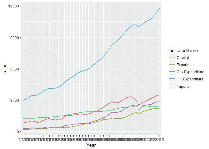
![The US’s GDP components (expenditure approach).]()
Figure 4.2 The US’s GDP components (expenditure approach).
There are plenty of problems with this chart:
- we cannot read the horizontal axis, because it labels every year
- the vertical axis label is uninformative
- there is no chart title
- the grey (default) background makes the chart difficult to read
- the legend is uninformative.
To improve this chart, we add features to the already existing figure
pl.pl = pl + scale_x_discrete(breaks=seq(1970, 2016, by = 10)) pl = pl + scale_y_continuous(name="Billion US$") pl = pl + ggtitle("GDP components over time") # Change the legend title and labels pl = pl + scale_colour_discrete(name = "Components of GDP", labels = c("Gross capital formation", "Exports", "Government expenditure", "Household expenditure", "Imports")) pl = pl + theme_bw() pl = pl + annotate("text", x = 37, y = 850, label = "Great Recession") pl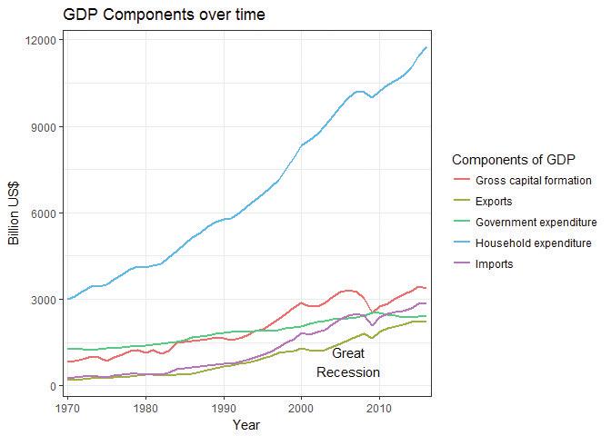
![The US’s GDP components (expenditure approach), amended chart.]()
Figure 4.3 The US’s GDP components (expenditure approach), amended chart.
We can make a chart for more than one country simultaneously by repeating the code above, but without subsetting the data:
# Repeat all steps without subsetting the data

# Base line chart
pl = ggplot(comp, aes(x = Year, y = value,
  color = IndicatorName))
pl = pl + geom_line(aes(group = IndicatorName), size = 1)
pl = pl + scale_x_discrete(
  breaks = seq(1970, 2016, by = 10))
pl = pl + scale_y_continuous(name = "Billion US$")
pl = pl + ggtitle("GDP components over time")
pl = pl + scale_colour_discrete(name = "Component")
pl = pl + theme_bw()

# Make a separate chart for each country
pl = pl + facet_wrap(~Country)
pl = pl + scale_colour_discrete(
  name = "Components of GDP",
  labels = c("Gross capital formation",
    "Exports",
    "Government expenditure",
    "Household expenditure",
    "Imports"))
pl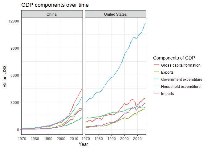
![GDP components over time (China and the US).]()
Figure 4.4 GDP components over time (China and the US).
- Another way to visualize the GDP data is to look at each component as a proportion of total GDP. Use the same countries that you chose for Question 3.
- For each country used in Question 3, create a new column showing the proportion of each component of total GDP (in other words, as a value ranging from 0 to 1). (Hint: to calculate the proportion of a component, divide the value of that component by the sum of all four components.)
- Plot a separate line chart for each country, showing the proportion of the component of GDP on the vertical axis and time (the years 1970 to the latest year available) on the horizontal axis.
- Describe any patterns in the proportion of spending over time for each country, and compare these patterns across countries.
- Compared to the charts in Question 3, what are some advantages of this method for making comparisons over time and between countries?
R walk-through 4.5 Calculating new variables and plotting time series data
Calculate proportion of total GDP
We will use the
compdataset created in R walk-through 4.4. First we will calculate net exports, as that contributes to GDP. As the data is currently in long format, we will reshape the data into wide format so that the variables we need are in separate columns instead of separate rows (using thedcastfunction, as in R walk-through 4.3), calculate net exports, then transform the data back into long format using themeltfunction.# Reshape the data to wide format (indicators in columns) comp_wide <- dcast(comp, Country + Year ~ IndicatorName) head(comp_wide)## Country Year Capital Exports Gov.Expenditure HH.Expenditure Imports ## 1 China 1970 67.58221 5.305242 19.30034 107.8411 6.119649 ## 2 China 1971 73.79977 6.318662 22.63929 112.3586 6.094361 ## 3 China 1972 70.62638 7.740001 23.77126 118.3906 7.510857 ## 4 China 1973 80.79658 10.810644 24.34177 126.7546 11.540975 ## 5 China 1974 83.38207 12.856408 26.14306 129.3434 16.041397 ## 6 China 1975 93.47130 13.309628 27.29335 134.5575 15.859461# Add the new column for net exports = exports – imports comp_wide$Net.Exports <- comp_wide[, "Exports"] - comp_wide[, "Imports"] head(comp_wide)## Country Year Capital Exports Gov.Expenditure HH.Expenditure Imports ## 1 China 1970 67.58221 5.305242 19.30034 107.8411 6.119649 ## 2 China 1971 73.79977 6.318662 22.63929 112.3586 6.094361 ## 3 China 1972 70.62638 7.740001 23.77126 118.3906 7.510857 ## 4 China 1973 80.79658 10.810644 24.34177 126.7546 11.540975 ## 5 China 1974 83.38207 12.856408 26.14306 129.3434 16.041397 ## 6 China 1975 93.47130 13.309628 27.29335 134.5575 15.859461 ## Net.Exports ## 1 -0.8144069 ## 2 0.2243011 ## 3 0.2291447 ## 4 -0.7303314 ## 5 -3.1849891 ## 6 -2.5498330# Return to long format with the HH.expenditure, Capital, and Net Export variables comp2_wide <- subset(comp_wide, select = -c(Exports, Imports)) comp2 <- melt(comp2_wide, id.vars = c("Year", "Country"))Now we will create a new dataframe (
props) also containing the proportions for each GDP component (proportion), using the piping operator to link functions together.props = comp2 %>% group_by(Country, Year) %>% mutate(proportion = value / sum(value))In words, we did the following: Take the
comp2dataframe and create groups by country and year (for example, all indicators for China in 1970). Then create a new variable (mutate) calledproportion, which divides the variablevalueof an indicator by the sum of allvaluefor that group (for example, all indicators for China in 1970). The result is then saved inprops. Look at thepropsdataframe to confirm that the above command has achieved the desired result.Plot a line chart
Now we redo the line chart from R walk-through 4.4 using the variable
props.# Base line chart pl = ggplot(props, aes(x = Year, y = proportion, color = variable)) pl = pl + geom_line(aes(group = variable), size = 1) pl = pl + scale_x_discrete(breaks = seq(1970, 2016, by = 10)) pl = pl + ggtitle("GDP component proportions over time") pl = pl + theme_bw() # Make a separate chart for each country pl = pl + facet_wrap(~Country) pl = pl + scale_colour_discrete( name = "Components of GDP", labels = c("Gross capital formation", "Government expenditure", "Household expenditure", "Net Exports")) pl
- time series data
- A time series is a set of time-ordered observations of a variable taken at successive, in most cases regular, periods or points of time. Example: The population of a particular country in the years 1990, 1991, 1992, … , 2015 is time series data.
- cross-sectional data
- Data that is collected from participants at one point in time or within a relatively short time frame. In contrast, time series data refers to data collected by following an individual (or firm, country, etc.) over a course of time. Example: Data on degree courses taken by all the students in a particular university in 2016 is considered cross-sectional data. In contrast, data on degree courses taken by all students in a particular university from 1990 to 2016 is considered time series data.
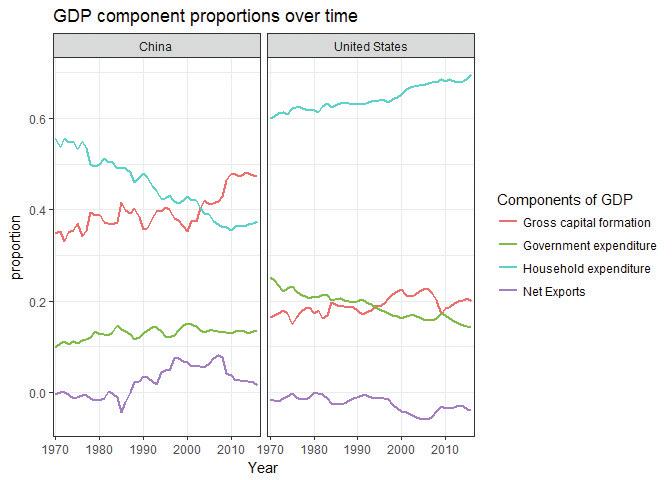
![GDP component proportions over time (China and the US).]()
Figure 4.5 GDP component proportions over time (China and the US).
So far, we have done comparisons of time series data, which is a collection of values for the same variables and subjects, taken at different points in time (for example, GDP of a particular country, measured each year). We will now make some charts using cross-sectional data, which is a collection of values for the same variables for different subjects, usually taken at the same time.
- Choose three developed countries, three countries in economic transition, and three developing countries (for a list of these countries, see Tables A–C in the UN country classification document).
- For each country, calculate each component as a proportion of GDP for the year 2015 only.
- Now create a stacked bar chart that shows the composition of GDP in 2015 on the horizontal axis, and country on the vertical axis. Arrange the columns so that the countries in a particular category are grouped together. (See the walk-through in Figure 3.8 of Economy, Society, and Public Policy for an example of what your chart should look like.)
- Describe the differences (if any) between the spending patterns of developed, economic transition, and developing countries.
R walk-through 4.6 Creating stacked bar charts
Calculate proportion of total GDP
This walk-through uses the following countries (chosen for purposes of illustration):
- developed countries: Germany, Japan, United States
- transition countries: Albania, Russian Federation, Ukraine
- developing countries: Brazil, China, India.
The relevant data are still in the
table_UNdataframe. Before we select these countries, we first calculate the required proportions for all countries.# Calculate proportions table_UN$p_Capital <- table_UN$Capital / (table_UN$Capital + table_UN$Final.Expenditure + table_UN$Net.Exports) table_UN$p_FinalExp <- table_UN$Final.Expenditure / (table_UN$Capital + table_UN$Final.Expenditure + table_UN$Net.Exports) table_UN$p_NetExports <- table_UN$Net.Exports / (table_UN$Capital + table_UN$Final.Expenditure + table_UN$Net.Exports) sel_countries <- c("Germany", "Japan", "United States", "Albania", "Russian Federation", "Ukraine", "Brazil", "China", "India") # Using our long format dataset, we select imports, # exports, and year for our chosen countries in 2015. # Select the columns we need sel_2015 <- subset(table_UN, subset = (Country %in% sel_countries) & (Year == 2015), select = c("Country", "Year", "p_FinalExp", "p_Capital", "p_NetExports"))Plot a stacked bar chart
Now let’s create the bar chart.
# Reshape the table into long format, then use ggplot
sel_2015_m <- melt(sel_2015, id.vars =
  c("Year", "Country"))

g <- ggplot(sel_2015_m,
  aes(x = Country, y = value, fill = variable)) +
  geom_bar(stat = "identity") + coord_flip() +
  ggtitle("GDP component proportions in 2015") +
  scale_fill_discrete(name = "Components of GDP",
  labels = c("Final expenditure",
    "Gross capital formation",
    "Net Exports")) +
  theme_bw()

plot(g)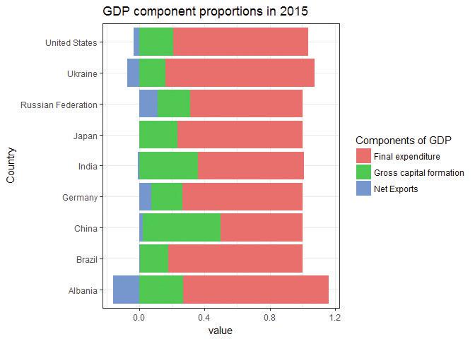
![GDP component proportions in 2015.]()
Figure 4.6 GDP component proportions in 2015.
Note that even when a country has a trade deficit (proportion of net exports < 0), the proportions will add up to 1, but the proportions of final expenditure and capital will add up to more than 1.
We have not yet ordered the countries so that they form the pre-specified groups. To achieve this, we need to explicitly impose an ordering on the
Countryvariable using thefactorfunction. The countries will be ordered in the same order we used to definesel_countries.# Impose the order in the sel_countries object, then use ggplot sel_2015_m$Country <- factor(sel_2015_m$Country, levels = sel_countries) g <- ggplot(sel_2015_m, aes(x = Country, y = value, fill = variable)) + geom_bar(stat = "identity") + coord_flip() + ggtitle("GDP component proportions in 2015 (ordered)") + scale_fill_discrete(name = "Components of GDP", labels = c("Final expenditure", "Gross capital formation", "Net Exports")) + theme_bw() plot(g)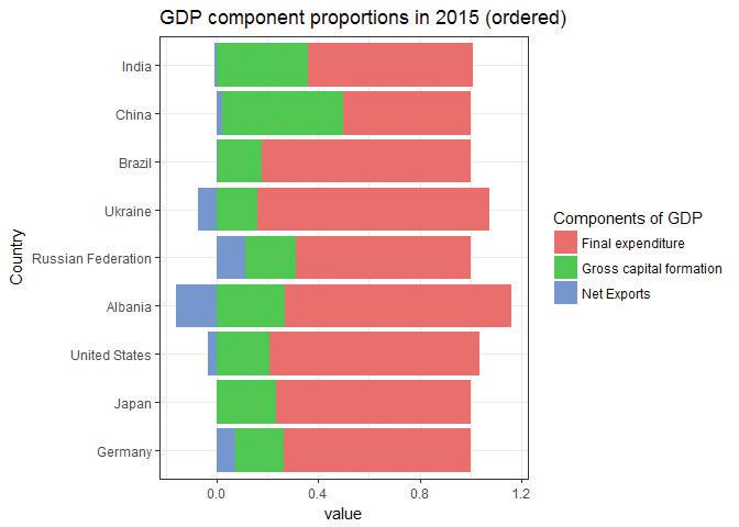
![GDP component proportions in 2015 (ordered).]()
Figure 4.7 GDP component proportions in 2015 (ordered).
-
GDP per capita is often used to indicate material wellbeing instead of GDP, because it accounts for differences in population across countries. Refer to the following articles to help you to answer the questions:
- ‘The Economics of Well-being’ in the Harvard Business Review
- ‘Statistical Insights: What does GDP per capita tell us about households’ material well-being?’ in the OECD Insights.
- Discuss the usefulness and limitations of GDP per capita as a measure of material wellbeing.
- Based on the arguments in the articles, do you think GDP per capita is an appropriate measure of both material wellbeing and overall wellbeing? Why or why not?
Part 4.2 The HDI as a measure of wellbeing
Learning objectives for this part
- Sort data and assign ranks based on values.
- Distinguish between time series and cross sectional data, and plot appropriate charts for each type of data.
- Calculate the geometric mean and explain how it differs from the arithmetic mean.
- Construct indices using the geometric mean, and use index values to rank observations.
- Explain the difference between two measures of wellbeing (GDP per capita and the Human Development Index).
In Part 4.1 we looked at GDP per capita as a measure of material wellbeing. While income has a major influence on wellbeing because it allows us to buy the goods and services we need or enjoy, it is not the only determinant of wellbeing. Many aspects of our wellbeing cannot be bought, for example, good health or having more time to spend with friends and family.
We are now going to look at the Human Development Index (HDI), a measure of wellbeing that includes non-material aspects, and make comparisons with GDP per capita (a measure of material wellbeing). GDP per capita is a simple index calculated as the sum of its elements, whereas the HDI is more complex. Instead of using different types of expenditure or output to measure wellbeing or living standards, the HDI consists of three dimensions associated with wellbeing:
- a long and healthy life (health)
- knowledge (education)
- a decent standard of living (income).
We will first learn about how the HDI is constructed, and then use this method to construct indices of wellbeing according to criteria of our choice.
The HDI data we will look at is from the Human Development Report by the United Nations Development Programme (UNDP). To answer the questions below, download the data and technical notes from the report:
- Go to the UNDP’s website.
- Click ‘Table 1: Human Development Index and its components’ to download the HDI data as an Excel file.
- Save the file in an easily accessible location, and make sure to give it a suitable name.
- The ‘Technical notes’ give a diagrammatic presentation of how the HDI is constructed from four indicators.
- Refer to the technical notes and the spreadsheet you have downloaded. For each indicator, explain whether you think it is a good measure of the dimension, and suggest alternative indicators, if any. (For example, is GNI per capita a good measure of the dimension ‘a decent standard of living’?)
- Figure 4.8 shows the minimum and maximum values for each indicator. Discuss whether you think these are reasonable. (You can read the justification for these values in the technical notes.)
| Dimension | Indicator | Minimum | Maximum |
|---|---|---|---|
| Health | Life expectancy (years) | 20 | 85 |
| Education | Expected years of schooling (years) | 0 | 18 |
| Mean years of schooling (years) | 0 | 15 | |
| Standard of living | Gross national income per capita (2011 PPP $) | 100 | 75,000 |
Figure 4.8 Maximum and minimum values for each indicator in the HDI.
United Nations Development Programme. 2022. ‘Technical notes’ in Human Development Report 2021/22: p. 2.
We are now going to apply the method for constructing the HDI, by recalculating the HDI from its indicators. We will use the formula below, and the minimum and maximum values in the table in Figure 4.8. These are taken from page 2 of the technical notes, which you can refer to for additional details.
The HDI indicators are measured in different units and have different ranges, so in order to put them together into a meaningful index, we need to normalize the indicators using the following formula:
\[\text{Dimension index } = \frac{\text{actual value − minimum value}}{\text{maximum value − minimum value}}\]Doing so will give a value in between 0 and 1 (inclusive), which will allow comparison between different indicators.
- Refer to Figure 4.8 and calculate the dimension index for each of the dimensions:
- Using the HDI indicator data in Column E of the spreadsheet, calculate the dimension index for a long and healthy life (health).
- Using the HDI indicator data in Columns G and I of the spreadsheet, calculate the dimension index for knowledge (education). Note that the knowledge dimension index is the average of the dimension index for expected years of schooling for those entering school, and mean years of schooling for adults aged 25 or older. When calculating the index for expected years of schooling you need to restrict the values to take a maximum value of 1.
- Using the HDI indicator data in Column K of the spreadsheet, calculate the dimension index for a decent standard of living (income). Note (from the technical notes) that you should calculate the GNI index using the natural log of the values. (See the ‘Find out more’ box below for an explanation of the natural log and how to calculate it in R.)
Find out more The natural log: What it means, and how to calculate it in R
The natural log turns a linear variable into a concave variable, as shown in Figure 4.9. For any value of income on the horizontal axis, the natural log of that value on the vertical axis is smaller. At first, the difference between income and log income is not that big (for example, an income of 2 corresponds to a natural log of 0.7), but the difference becomes bigger as we move rightwards along the horizontal axis (for example, when income is 100,000, the natural log is only 11.5).
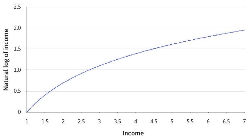
![Comparing income with the natural logarithm of income.]()
Figure 4.9 Comparing income with the natural logarithm of income.
The reason why natural logs are useful in economics is because they can represent variables that have diminishing marginal returns: an additional unit of input results in a smaller increase in the total output than did the previous unit. (If you have studied production functions, then the shape of the natural log function might look familiar.)
When applied to the concept of wellbeing, the ‘input’ is income, and the ‘output’ is material wellbeing. It makes intuitive sense that a $100 increase in per capita income will have a much greater effect on wellbeing for a poor country compared to a rich country. Using the natural log of income incorporates this notion into the index we create. Conversely, the notion of diminishing marginal returns (the larger the value of the input, the smaller the contribution of an additional unit of input) is not captured by GDP per capita, which uses actual income and not its natural log. Doing so makes the assumption that a $100 increase in per capita income has the same effect on wellbeing for rich and poor countries.
The
logfunction in R calculates the natural log of a value for you. To calculate the natural log of a value, x, typelog(x). If you have a scientific calculator, you can check that the calculation is correct by using thelnorlogkey.Now that you know about the natural log, you might want to go back to Question 3(c) in Part 4.1, and create a new chart using the natural log scale. The natural log is used in economics because it approximates percentage changes i.e. log(x) – log(y) is a close approximation to the percentage change between x and y. So, using the natural log scale, you will be able to ‘read off’ the relative growth rates from the slopes of the different series you have plotted. For example, a 0.01 change in the vertical axis value corresponds to a 1% change in that variable. This will allow you to compare the growth rates of the different components of GDP.
- geometric mean
- A summary measure calculated by multiplying N numbers together and then taking the Nth root of this product. The geometric mean is useful when the items being averaged have different scoring indices or scales, because it is not sensitive to these differences, unlike the arithmetic mean. For example, if education ranged from 0 to 20 years and life expectancy ranged from 0 to 85 years, life expectancy would have a bigger influence on the HDI than education if we used the arithmetic mean rather than the geometric mean. Conversely, the geometric mean treats each criteria equally. Example: Suppose we use life expectancy and mean years of schooling to construct an index of wellbeing. Country A has life expectancy of 40 years and a mean of 6 years of schooling. If we used the arithmetic mean to make an index, we would get (40 + 6)/2 = 23. If we used the geometric mean, we would get (40 × 6)1/2 = 15.5. Now suppose life expectancy doubled to 80 years. The arithmetic mean would be (80 + 6)/2 = 43, and the geometric mean would be (80 × 6)1/2 = 21.9. If, instead, mean years of schooling doubled to 12 years, the arithmetic mean would be (40 + 12)/2 = 26, and the geometric mean would be (40 × 12)1/2 = 21.9. This example shows that the arithmetic mean can be ‘unfair’ because proportional changes in one variable (life expectancy) have a larger influence over the index than changes in the other variable (years of schooling). The geometric mean gives each variable the same influence over the value of the index, so doubling the value of one variable would have the same effect on the index as doubling the value of another variable.
Now, we can combine these dimensional indices to give the HDI. The HDI is the geometric mean of the three dimension indices (IHealth = Life expectancy index, IEducation = Education index, and IIncome = GNI index):
\[\text{HDI }=(\text{I}_{\text{Health}} \times \text{I}_{\text{Education}} \times \text{I}_{\text{Income}})^{1/3}\]- Use the formula above and the data in the spreadsheet to calculate the HDI for all the countries excluding those in the ‘Other countries or territories’ category. You should get the same values as those in Column C, rounded to three decimal places.
R walk-through 4.7 Calculating the HDI
We will use
read_excelto import the data file, which we saved as ‘HDR_data.xlsx’ in our working directory. Before importing, look at the Excel file so that you understand its structure and how it corresponds to the code options used below. We will save the imported data as the dataframeHDR2021.# File path HDR2021 <- read_excel("HDR_data.xlsx", # Worksheet to import sheet = "Table 1", # Number of rows to skip skip = 3) head(HDR2021)## # A tibble: 6 × 15 ## ...1 ...2 Human…¹ ...4 Life …² ...6 Expec…³ ...8 Mean …⁴ ...10 Gross…⁵ ## <chr> <chr> <chr> <lgl> <chr> <chr> <chr> <chr> <chr> <chr> <chr> ## 1 HDI rank Coun… Value NA (years) <NA> (years) <NA> (years) <NA> (2017 … ## 2 <NA> <NA> 2021 NA 2021 <NA> 2021 a 2021 a 2021 ## 3 <NA> VERY… <NA> NA <NA> <NA> <NA> <NA> <NA> <NA> <NA> ## 4 1 Swit… 0.9619… NA 83.987… <NA> 16.500… <NA> 13.859… <NA> 66933.… ## 5 2 Norw… 0.9609… NA 83.233… <NA> 18.185… c 13.003… <NA> 64660.… ## 6 3 Icel… 0.9589… NA 82.678… <NA> 19.163… c 13.767… <NA> 55782.… ## # … with 4 more variables: ...12 <chr>, ## # `GNI per capita rank minus HDI rank` <chr>, ...14 <chr>, `HDI rank` <chr>, ## # and abbreviated variable names ¹`Human Development Index (HDI)`, ## # ²`Life expectancy at birth`, ³`Expected years of schooling`, ## # ⁴`Mean years of schooling`, ⁵`Gross national income (GNI) per capita`str(HDR2021)## tibble [272 × 15] (S3: tbl_df/tbl/data.frame) ## $ ...1 : chr [1:272] "HDI rank" NA NA "1" ... ## $ ...2 : chr [1:272] "Country" NA "VERY HIGH HUMAN DEVELOPMENT" "Switzerland" ... ## $ Human Development Index (HDI) : chr [1:272] "Value" "2021" NA "0.96199999999999997" ... ## $ ...4 : logi [1:272] NA NA NA NA NA NA ... ## $ Life expectancy at birth : chr [1:272] "(years)" "2021" NA "83.987200000000001" ... ## $ ...6 : chr [1:272] NA NA NA NA ... ## $ Expected years of schooling : chr [1:272] "(years)" "2021" NA "16.50029945" ... ## $ ...8 : chr [1:272] NA "a" NA NA ... ## $ Mean years of schooling : chr [1:272] "(years)" "2021" NA "13.85966015" ... ## $ ...10 : chr [1:272] NA "a" NA NA ... ## $ Gross national income (GNI) per capita: chr [1:272] "(2017 PPP $)" "2021" NA "66933.004539999994" ... ## $ ...12 : chr [1:272] NA NA NA NA ... ## $ GNI per capita rank minus HDI rank : chr [1:272] NA "2021" NA "5" ... ## $ ...14 : chr [1:272] NA "b" NA NA ... ## $ HDI rank : chr [1:272] NA "2020" NA "3" ...Looking at the
HDRdataframe, there are rows that have information that isn’t data (for example, all the rows with an ‘NA’ in the first column), as well as variables/columns that do not contain data (for example, most columns beginning with a ‘…’, though columns labelled...1and...2contain the HDI rank and the country names respectively).Cleaning up the dataframe can be easier to do in Excel by deleting irrelevant rows and columns, but one advantage of doing it in R is replicability. Suppose in a year’s time you carried out the analysis again with an updated spreadsheet containing new information. If you had done the cleaning in Excel, you would have to redo it from scratch, but if you had done it in R, you can simply rerun the code below.
Firstly, we eliminate rows that do not have any numbers in the
HDI rankcolumn (or...1).# Rename the first column, currently named ...1 names(HDR2021)[1] <- "HDI.rank" # Rename the second column, currently named ...2 names(HDR2021)[2] <- "Country" # Rename the last column, which contains the 2020 rank names(HDR2021)[names(HDR2021) == "HDI rank"] <- "HDI.rank.2020" # Eliminate the row that contains the column title HDR2021 <- subset(HDR2021, !is.na(HDI.rank) & HDI.rank != "HDI rank")Then we eliminate columns that contain notes in the original spreadsheet (names starting with ‘…’).
# Check which variables do NOT (!) start with '...'
sel_columns <- !startsWith(names(HDR2021), "...")

# Select the columns that do not start with '...'
HDR2021 <- subset(HDR2021, select = sel_columns)

str(HDR2021)
## tibble [191 × 9] (S3: tbl_df/tbl/data.frame) ## $ HDI.rank : chr [1:191] "1" "2" "3" "4" ... ## $ Country : chr [1:191] "Switzerland" "Norway" "Iceland" "Hong Kong, China (SAR)" ... ## $ Human Development Index (HDI) : chr [1:191] "0.96199999999999997" "0.96099999999999997" "0.95899999999999996" "0.95199999999999996" ... ## $ Life expectancy at birth : chr [1:191] "83.987200000000001" "83.233900000000006" "82.678200000000004" "85.473399999999998" ... ## $ Expected years of schooling : chr [1:191] "16.50029945" "18.185199740000002" "19.163059230000002" "17.278169630000001" ... ## $ Mean years of schooling : chr [1:191] "13.85966015" "13.00362968" "13.76716995" "12.22620964" ... ## $ Gross national income (GNI) per capita: chr [1:191] "66933.004539999994" "64660.106220000001" "55782.049809999997" "62606.845399999998" ... ## $ GNI per capita rank minus HDI rank : chr [1:191] "5" "6" "11" "6" ... ## $ HDI.rank.2020 : chr [1:191] "3" "1" "2" "4" ...Let’s change some of the long variable names (those in columns 3–8) to shorter ones.
names(HDR2021)[3] <- "HDI"
names(HDR2021)[4] <- "LifeExp"
names(HDR2021)[5] <- "ExpSchool"
names(HDR2021)[6] <- "MeanSchool"
names(HDR2021)[7] <- "GNI.capita"
names(HDR2021)[8] <- "GNI.HDI.rank"
Looking at the structure of the data, we see that R thinks that all the data are
chr(character or text variables) because the original datafile contained non-numerical entries (these rows have now been deleted). Apart from theCountryvariable, which we want to be a factor variable (containing categories), all variables should be numeric.HDR2021$HDI.rank <- as.numeric(HDR2021$HDI.rank) HDR2021$Country <- as.factor(HDR2021$Country) HDR2021$HDI <- as.numeric(HDR2021$HDI) HDR2021$LifeExp <- as.numeric(HDR2021$LifeExp) HDR2021$ExpSchool <- as.numeric(HDR2021$ExpSchool) HDR2021$MeanSchool <- as.numeric(HDR2021$MeanSchool) HDR2021$GNI.capita <- as.numeric(HDR2021$GNI.capita) HDR2021$GNI.HDI.rank <- as.numeric(HDR2021$GNI.HDI.rank) HDR2021$HDI.rank.2020 <- as.numeric(HDR2021$HDI.rank.2020) str(HDR2021)## tibble [191 × 9] (S3: tbl_df/tbl/data.frame) ## $ HDI.rank : num [1:191] 1 2 3 4 5 6 7 8 9 10 ... ## $ Country : Factor w/ 191 levels "Afghanistan",..: 166 128 77 75 9 47 165 82 65 122 ... ## $ HDI : num [1:191] 0.962 0.961 0.959 0.952 0.951 0.948 0.947 0.945 0.942 0.941 ... ## $ LifeExp : num [1:191] 84 83.2 82.7 85.5 84.5 ... ## $ ExpSchool : num [1:191] 16.5 18.2 19.2 17.3 21.1 ... ## $ MeanSchool : num [1:191] 13.9 13 13.8 12.2 12.7 ... ## $ GNI.capita : num [1:191] 66933 64660 55782 62607 49238 ... ## $ GNI.HDI.rank : num [1:191] 5 6 11 6 18 6 9 -3 6 3 ... ## $ HDI.rank.2020: num [1:191] 3 1 2 4 5 5 9 8 7 10 ...Now we have a nice clean dataset that we can work with.
We start by calculating the three indices, using the information given. For the education index we calculate the index for expected and mean schooling separately, then take the arithmetic mean to get
I.Education. As some mean schooling observations exceed the specified ‘maximum’ value of 18, the calculated index values would be larger than 1. To avoid this, we usepminto replace these observations with 18 to obtain an index value of 1.HDR2021$I.Health <- (HDR2021$LifeExp - 20) / (85 - 20) HDR2021$I.Education <- ((pmin(HDR2021$ExpSchool, 18) - 0) / (18 - 0) + (HDR2021$MeanSchool - 0) / (15 - 0)) / 2 HDR2021$I.Income <- (log(HDR2021$GNI.capita) - log(100)) / (log(75000) - log(100)) HDR2021$HDI.calc <- (HDR2021$I.Health * HDR2021$I.Education * HDR2021$I.Income)^(1/3)Now we can compare the
HDIgiven in the table and our calculated HDI.HDR2021[, c("HDI", "HDI.calc")]## # A tibble: 191 × 2 ## HDI HDI.calc ## <dbl> <dbl> ## 1 0.962 0.962 ## 2 0.961 0.961 ## 3 0.959 0.959 ## 4 0.952 0.954 ## 5 0.951 0.951 ## 6 0.948 0.948 ## 7 0.947 0.947 ## 8 0.945 0.946 ## 9 0.942 0.942 ## 10 0.941 0.941 ## # … with 181 more rows
The HDI is one way to measure wellbeing, but you may think that it does not use the most appropriate measures for the non-material aspects of wellbeing (health and education).
Now we will use the same method to create our own index of non-material wellbeing (an ‘alternative HDI’), using different indicators. You can find alternative indicators to measure health and education from the World Bank’s World Development Indicators. Use the interactive menu on the left to select and download alternative indicators of health and education:
- In the ‘Country’ section, click the tick box to select all countries.
- In the ‘Time’ section, click the tick box to select all available years.
- In the ‘Series’ section, find and select two or three indicators to measure health, and two to three indicators to measure education (check R walk-through 4.8 for some ideas). Also select the series ‘GNI per capita (constant 2015 US$)’, which we’ll use for the income indicator.
- Minimise all sections in the left-side menu. Then click ‘Apply Changes’ to preview the data.
- Click ‘Download options’ (near the top of the page) and select ‘CSV’ to download the data as a .csv file.
- The data will download as a .zip file containing two .csv files. The first file, with ‘Data.csv’ in the filename, contains the indicators we need. Save this file in your ‘data’ subfolder and give it an easy-to-remember name (like ‘world_bank_data.csv’).
- Create an alternative index of wellbeing. In particular, propose alternative Education and Health indices in (a) and (b), then combine these with the alternative Income index in (c) to calculate an alternative HDI. Examine whether the changes caused substantial changes in country rankings in (d).
- Choose two to three indicators to measure health, and two to three indicators to measure education. Explain why you have chosen these indicators.
- Choose a reasonable maximum and minimum value for each indicator and justify your choices.
- Calculate your alternative versions of the education and health dimension indices. Since you have chosen more than one indicator for this dimension, make sure to average the dimension indices as done in Question 3(b). Also ensure that higher indicator values always represent better outcomes. Now calculate the alternative HDI as done in Questions 3 and 4. Remember to combine your alternative education and health indices with the existing income index from Question 2.
- Create a new variable showing each country’s rank according to your alternative HDI, where 1 is assigned to the country with the highest value. Compare your ranking to the HDI rank. Are the rankings generally similar, or very different? (See R walk-through 4.8 on how to do this.)
R walk-through 4.8 Creating your own HDI
Merge data and calculate alternative indices
This example uses the following indicators:
Education: School enrollment, tertiary (% gross); Trained teachers in primary education (% of total teachers). Health: Mortality rate, adult, female (per 1,000 female adults); Mortality rate, adult, male (per 1,000 male adults). Income: GNI per capita (in constant 2015 USD). If you’re using different indicators, remember to adjust the code below accordingly.
First, we import the data, which we saved as
world_bank_data.csv, and check that it has been imported correctly. You can see that each row represents a different country, and each column represents a different year–indicator combination. Note that the data comes with some empty rows at the end before some metadata that has been inserted (information about where the data came from and the download date). To remove the metadata, we drop these rows.all_hdr <- read.csv("world_bank_data.csv") head(all_hdr)## Country.Name Country.Code ## 1 Afghanistan AFG ## 2 Afghanistan AFG ## 3 Afghanistan AFG ## 4 Afghanistan AFG ## 5 Afghanistan AFG ## 6 Albania ALB ## Series.Name Series.Code ## 1 School enrollment, tertiary (% gross) SE.TER.ENRR ## 2 Trained teachers in primary education (% of total teachers) SE.PRM.TCAQ.ZS ## 3 Mortality rate, adult, female (per 1,000 female adults) SP.DYN.AMRT.FE ## 4 Mortality rate, adult, male (per 1,000 male adults) SP.DYN.AMRT.MA ## 5 GNI per capita (constant 2015 US$) NY.GNP.PCAP.KD ## 6 School enrollment, tertiary (% gross) SE.TER.ENRR ## X1960..YR1960. X1961..YR1961. X1962..YR1962. X1963..YR1963. X1964..YR1964. ## 1 .. .. .. .. .. ## 2 .. .. .. .. .. ## 3 550.189 543.6 537.703 531.856 526.179 ## 4 601.887 594.812 588.87 583.144 577.178 ## 5 .. .. .. .. .. ## 6 .. .. .. .. .. ## X1965..YR1965. X1966..YR1966. X1967..YR1967. X1968..YR1968. X1969..YR1969. ## 1 .. .. .. .. .. ## 2 .. .. .. .. .. ## 3 520.698 514.339 508.496 502.464 496.613 ## 4 571.526 565.571 559.967 554.061 548.058 ## 5 .. .. .. .. .. ## 6 .. .. .. .. .. ## X1970..YR1970. X1971..YR1971. X1972..YR1972. X1973..YR1973. X1974..YR1974. ## 1 0.806509972 0.977230012 1.014490008 1.171839952 1.097650051 ## 2 .. .. .. .. .. ## 3 490.203 483.941 477.325 470.742 464.507 ## 4 542.163 536.333 530.118 523.162 516.322 ## 5 .. .. .. .. .. ## 6 .. 11.99890995 12.76107025 .. .. ## X1975..YR1975. X1976..YR1976. X1977..YR1977. X1978..YR1978. X1979..YR1979. ## 1 1.193840027 1.348080039 1.495440006 1.908800006 2.033169985 ## 2 .. .. .. .. .. ## 3 458.609 452.685 446.568 453.421 462.727 ## 4 509.418 502.722 495.365 536.287 580.634 ## 5 .. .. .. .. .. ## 6 .. .. .. 4.794219971 .. ## X1980..YR1980. X1981..YR1981. X1982..YR1982. X1983..YR1983. X1984..YR1984. ## 1 .. .. 2.190550089 .. .. ## 2 .. .. .. .. .. ## 3 456.101 449.554 471.749 465.209 515.459 ## 4 575.356 570.111 642.693 641.458 762.193 ## 5 .. .. .. .. .. ## 6 .. 4.322169781 .. 5.104380131 5.764540195 ## X1985..YR1985. X1986..YR1986. X1987..YR1987. X1988..YR1988. X1989..YR1989. ## 1 .. 2.379489899 1.881790042 .. .. ## 2 .. .. .. .. .. ## 3 511.766 448.188 442.407 401.952 390.109 ## 4 764.443 639.184 637.127 542.567 521.198 ## 5 .. .. .. .. .. ## 6 6.306069851 6.600470066 6.813399792 7.329929829 7.871230125 ## X1990..YR1990. X1991..YR1991. X1992..YR1992. X1993..YR1993. X1994..YR1994. ## 1 2.465280056 .. .. .. .. ## 2 .. .. .. .. .. ## 3 382.051 373.966 362.387 333.348 326.338 ## 4 510.052 502.877 499.627 393.724 422.588 ## 5 .. .. .. .. .. ## 6 8.223870277 8.84414959 9.196969986 10.98034954 10.36900043 ## X1995..YR1995. X1996..YR1996. X1997..YR1997. X1998..YR1998. X1999..YR1999. ## 1 .. .. .. .. .. ## 2 .. .. .. .. .. ## 3 319.863 311.9 308.249 316.547 295.841 ## 4 390.447 381.229 374.88 401.359 357.328 ## 5 .. .. .. .. .. ## 6 9.962510109 10.82717037 12.5855999 13.40367031 14.53652 ## X2000..YR2000. X2001..YR2001. X2002..YR2002. X2003..YR2003. X2004..YR2004. ## 1 .. .. .. 1.381070018 1.389660001 ## 2 .. .. .. .. .. ## 3 290.083 284.871 282.338 270.723 264.795 ## 4 355.447 349.36 331.54 321.913 313.483 ## 5 .. .. .. .. .. ## 6 15.23215961 15.49168015 15.93058968 16.38154984 19.82195091 ## X2005..YR2005. X2006..YR2006. X2007..YR2007. X2008..YR2008. X2009..YR2009. ## 1 .. .. .. .. 4.024809837 ## 2 .. .. .. .. .. ## 3 259.868 254.511 247.96 241.256 236.917 ## 4 310.94 314.837 318.012 305.06 293.605 ## 5 .. .. .. .. .. ## 6 23.53915024 27.70500946 32.11925888 33.41545105 34.2157402 ## X2010..YR2010. X2011..YR2011. X2012..YR2012. X2013..YR2013. X2014..YR2014. ## 1 .. 3.755609989 .. .. 8.310870171 ## 2 .. .. .. .. .. ## 3 231.583 225.563 220.219 214.871 212.215 ## 4 288.75 282.654 277.057 271.596 274.007 ## 5 .. .. .. .. .. ## 6 45.00257874 49.66601181 59.5761795 65.31529236 66.82601166 ## X2015..YR2015. X2016..YR2016. X2017..YR2017. X2018..YR2018. X2019..YR2019. ## 1 .. .. .. 9.96378994 .. ## 2 .. .. .. .. .. ## 3 209.573 204.096 196.522 193.284 190.261 ## 4 278.424 274.045 311.655 319.849 305.768 ## 5 597.8323206 .. .. .. .. ## 6 62.98656082 59.27449036 58.65351105 56.60887146 62.07609177 ## X2020..YR2020. X2021..YR2021. X2022..YR2022. ## 1 10.8584404 .. .. ## 2 .. .. .. ## 3 210.053 214.241 .. ## 4 318.587 342.158 .. ## 5 .. .. .. ## 6 61.39257813 60.31758118 62.73199081tail(all_hdr) # the last 5 rows are "empty"## Country.Name Country.Code ## 1330 World WLD ## 1331 ## 1332 ## 1333 ## 1334 Data from database: World Development Indicators ## 1335 Last Updated: 10/26/2023 ## Series.Name Series.Code X1960..YR1960. ## 1330 GNI per capita (constant 2015 US$) NY.GNP.PCAP.KD .. ## 1331 ## 1332 ## 1333 ## 1334 ## 1335 ## X1961..YR1961. X1962..YR1962. X1963..YR1963. X1964..YR1964. X1965..YR1965. ## 1330 .. .. .. .. .. ## 1331 ## 1332 ## 1333 ## 1334 ## 1335 ## X1966..YR1966. X1967..YR1967. X1968..YR1968. X1969..YR1969. X1970..YR1970. ## 1330 .. .. .. .. .. ## 1331 ## 1332 ## 1333 ## 1334 ## 1335 ## X1971..YR1971. X1972..YR1972. X1973..YR1973. X1974..YR1974. X1975..YR1975. ## 1330 .. .. .. .. .. ## 1331 ## 1332 ## 1333 ## 1334 ## 1335 ## X1976..YR1976. X1977..YR1977. X1978..YR1978. X1979..YR1979. X1980..YR1980. ## 1330 .. .. .. .. .. ## 1331 ## 1332 ## 1333 ## 1334 ## 1335 ## X1981..YR1981. X1982..YR1982. X1983..YR1983. X1984..YR1984. X1985..YR1985. ## 1330 6174.90648 6074.020218 6141.672396 6313.05707 6426.580209 ## 1331 ## 1332 ## 1333 ## 1334 ## 1335 ## X1986..YR1986. X1987..YR1987. X1988..YR1988. X1989..YR1989. X1990..YR1990. ## 1330 6513.715752 6638.760978 6812.636836 6962.734089 7008.565071 ## 1331 ## 1332 ## 1333 ## 1334 ## 1335 ## X1991..YR1991. X1992..YR1992. X1993..YR1993. X1994..YR1994. X1995..YR1995. ## 1330 6978.677125 6974.742139 6949.376323 7033.451963 7112.311336 ## 1331 ## 1332 ## 1333 ## 1334 ## 1335 ## X1996..YR1996. X1997..YR1997. X1998..YR1998. X1999..YR1999. X2000..YR2000. ## 1330 7255.341713 7429.262588 7538.518418 7713.722339 7949.373184 ## 1331 ## 1332 ## 1333 ## 1334 ## 1335 ## X2001..YR2001. X2002..YR2002. X2003..YR2003. X2004..YR2004. X2005..YR2005. ## 1330 8005.710503 8066.305932 8217.561083 8471.396397 8693.154115 ## 1331 ## 1332 ## 1333 ## 1334 ## 1335 ## X2006..YR2006. X2007..YR2007. X2008..YR2008. X2009..YR2009. X2010..YR2010. ## 1330 8963.788753 9234.913447 9288.601877 9050.092114 9344.137572 ## 1331 ## 1332 ## 1333 ## 1334 ## 1335 ## X2011..YR2011. X2012..YR2012. X2013..YR2013. X2014..YR2014. X2015..YR2015. ## 1330 9532.88803 9666.326486 9806.347742 10001.55659 10177.03967 ## 1331 ## 1332 ## 1333 ## 1334 ## 1335 ## X2016..YR2016. X2017..YR2017. X2018..YR2018. X2019..YR2019. X2020..YR2020. ## 1330 10336.6271 10579.83371 10796.97748 10975.7017 10500.28598 ## 1331 ## 1332 ## 1333 ## 1334 ## 1335 ## X2021..YR2021. X2022..YR2022. ## 1330 11044.61837 .. ## 1331 ## 1332 ## 1333 ## 1334 ## 1335all_hdr = all_hdr[-((nrow(all_hdr)-4):nrow(all_hdr)),] str(all_hdr)## 'data.frame': 1330 obs. of 67 variables: ## $ Country.Name : chr "Afghanistan" "Afghanistan" "Afghanistan" "Afghanistan" ... ## $ Country.Code : chr "AFG" "AFG" "AFG" "AFG" ... ## $ Series.Name : chr "School enrollment, tertiary (% gross)" "Trained teachers in primary education (% of total teachers)" "Mortality rate, adult, female (per 1,000 female adults)" "Mortality rate, adult, male (per 1,000 male adults)" ... ## $ Series.Code : chr "SE.TER.ENRR" "SE.PRM.TCAQ.ZS" "SP.DYN.AMRT.FE" "SP.DYN.AMRT.MA" ... ## $ X1960..YR1960.: chr ".." ".." "550.189" "601.887" ... ## $ X1961..YR1961.: chr ".." ".." "543.6" "594.812" ... ## $ X1962..YR1962.: chr ".." ".." "537.703" "588.87" ... ## $ X1963..YR1963.: chr ".." ".." "531.856" "583.144" ... ## $ X1964..YR1964.: chr ".." ".." "526.179" "577.178" ... ## $ X1965..YR1965.: chr ".." ".." "520.698" "571.526" ... ## $ X1966..YR1966.: chr ".." ".." "514.339" "565.571" ... ## $ X1967..YR1967.: chr ".." ".." "508.496" "559.967" ... ## $ X1968..YR1968.: chr ".." ".." "502.464" "554.061" ... ## $ X1969..YR1969.: chr ".." ".." "496.613" "548.058" ... ## $ X1970..YR1970.: chr "0.806509972" ".." "490.203" "542.163" ... ## $ X1971..YR1971.: chr "0.977230012" ".." "483.941" "536.333" ... ## $ X1972..YR1972.: chr "1.014490008" ".." "477.325" "530.118" ... ## $ X1973..YR1973.: chr "1.171839952" ".." "470.742" "523.162" ... ## $ X1974..YR1974.: chr "1.097650051" ".." "464.507" "516.322" ... ## $ X1975..YR1975.: chr "1.193840027" ".." "458.609" "509.418" ... ## $ X1976..YR1976.: chr "1.348080039" ".." "452.685" "502.722" ... ## $ X1977..YR1977.: chr "1.495440006" ".." "446.568" "495.365" ... ## $ X1978..YR1978.: chr "1.908800006" ".." "453.421" "536.287" ... ## $ X1979..YR1979.: chr "2.033169985" ".." "462.727" "580.634" ... ## $ X1980..YR1980.: chr ".." ".." "456.101" "575.356" ... ## $ X1981..YR1981.: chr ".." ".." "449.554" "570.111" ... ## $ X1982..YR1982.: chr "2.190550089" ".." "471.749" "642.693" ... ## $ X1983..YR1983.: chr ".." ".." "465.209" "641.458" ... ## $ X1984..YR1984.: chr ".." ".." "515.459" "762.193" ... ## $ X1985..YR1985.: chr ".." ".." "511.766" "764.443" ... ## $ X1986..YR1986.: chr "2.379489899" ".." "448.188" "639.184" ... ## $ X1987..YR1987.: chr "1.881790042" ".." "442.407" "637.127" ... ## $ X1988..YR1988.: chr ".." ".." "401.952" "542.567" ... ## $ X1989..YR1989.: chr ".." ".." "390.109" "521.198" ... ## $ X1990..YR1990.: chr "2.465280056" ".." "382.051" "510.052" ... ## $ X1991..YR1991.: chr ".." ".." "373.966" "502.877" ... ## $ X1992..YR1992.: chr ".." ".." "362.387" "499.627" ... ## $ X1993..YR1993.: chr ".." ".." "333.348" "393.724" ... ## $ X1994..YR1994.: chr ".." ".." "326.338" "422.588" ... ## $ X1995..YR1995.: chr ".." ".." "319.863" "390.447" ... ## $ X1996..YR1996.: chr ".." ".." "311.9" "381.229" ... ## $ X1997..YR1997.: chr ".." ".." "308.249" "374.88" ... ## $ X1998..YR1998.: chr ".." ".." "316.547" "401.359" ... ## $ X1999..YR1999.: chr ".." ".." "295.841" "357.328" ... ## $ X2000..YR2000.: chr ".." ".." "290.083" "355.447" ... ## $ X2001..YR2001.: chr ".." ".." "284.871" "349.36" ... ## $ X2002..YR2002.: chr ".." ".." "282.338" "331.54" ... ## $ X2003..YR2003.: chr "1.381070018" ".." "270.723" "321.913" ... ## $ X2004..YR2004.: chr "1.389660001" ".." "264.795" "313.483" ... ## $ X2005..YR2005.: chr ".." ".." "259.868" "310.94" ... ## $ X2006..YR2006.: chr ".." ".." "254.511" "314.837" ... ## $ X2007..YR2007.: chr ".." ".." "247.96" "318.012" ... ## $ X2008..YR2008.: chr ".." ".." "241.256" "305.06" ... ## $ X2009..YR2009.: chr "4.024809837" ".." "236.917" "293.605" ... ## $ X2010..YR2010.: chr ".." ".." "231.583" "288.75" ... ## $ X2011..YR2011.: chr "3.755609989" ".." "225.563" "282.654" ... ## $ X2012..YR2012.: chr ".." ".." "220.219" "277.057" ... ## $ X2013..YR2013.: chr ".." ".." "214.871" "271.596" ... ## $ X2014..YR2014.: chr "8.310870171" ".." "212.215" "274.007" ... ## $ X2015..YR2015.: chr ".." ".." "209.573" "278.424" ... ## $ X2016..YR2016.: chr ".." ".." "204.096" "274.045" ... ## $ X2017..YR2017.: chr ".." ".." "196.522" "311.655" ... ## $ X2018..YR2018.: chr "9.96378994" ".." "193.284" "319.849" ... ## $ X2019..YR2019.: chr ".." ".." "190.261" "305.768" ... ## $ X2020..YR2020.: chr "10.8584404" ".." "210.053" "318.587" ... ## $ X2021..YR2021.: chr ".." ".." "214.241" "342.158" ... ## $ X2022..YR2022.: chr ".." ".." ".." ".." ...Now we need to arrange the data in the same format as the HDI data (one column per variable), so we can use the same code as R walk-through 4.7 to calculate the alternative HDI. We will use the year 2021 as there is more data available compared to later years (you may want to use a later year if you are working with the latest dataset).
Currently the dataframe
all_hdrhas several rows for a particular country and year (one for each indicator). As in R walk-through 4.3, we will reshape this data using thedcastfunction to ensure that we have only one row per country.long_hdr = all_hdr[c("Country.Name", "Series.Code", "X2021..YR2021.")] # keep data from 2021 only long_hdr[long_hdr==".."] <- NA # code missing data ("..") as "NA" allHDR2021 = dcast(long_hdr, Country.Name ~ Series.Code, value.var="X2021..YR2021.")Then we follow the same process as in R walk-through 4.7—cleaning the data, getting the data for the indicators we want, and giving each indicator a shorter name.
# Rename the first column, currently named ...1
names(allHDR2021)[1] <- "Country"

# Rename the columns with shorter variable names
names(allHDR2021)[2] <- "income"
names(allHDR2021)[3] <- "trained_teachers"
names(allHDR2021)[4] <- "enrollment"
names(allHDR2021)[5] <- "mortality_female"
names(allHDR2021)[6] <- "mortality_male"

# Change variables to numeric (numbers)
allHDR2021$Country <- as.factor(allHDR2021$Country)
allHDR2021$income <- as.numeric(allHDR2021$income)
allHDR2021$trained_teachers <- as.numeric(allHDR2021$trained_teachers)
allHDR2021$enrollment <- as.numeric(allHDR2021$enrollment)
allHDR2021$mortality_female <- as.numeric(allHDR2021$mortality_female)
allHDR2021$mortality_male <- as.numeric(allHDR2021$mortality_male)

str(allHDR2021)
## 'data.frame': 266 obs. of 6 variables: ## $ Country : Factor w/ 266 levels "Afghanistan",..: 1 2 3 4 5 6 7 8 9 10 ... ## $ income : num NA 1425 1717 4793 3856 ... ## $ trained_teachers: num NA NA 68.7 61.8 98.1 ... ## $ enrollment : num NA 8.85 NA 60.32 54.21 ... ## $ mortality_female: num 214.2 237.6 305.2 62.1 64 ... ## $ mortality_male : num 342.2 332.8 346.6 122.1 95.8 ...Looking at the structure (
str( )), we can see that all indicators are correctly in numerical (num) format.Before we can calculate indices, we need to set minimum and maximum values, which we base on the minimum and maximum values in the sample.
summary(allHDR2021)## Country income trained_teachers ## Afghanistan : 1 Min. : 265.3 Min. : 22.57 ## Africa Eastern and Southern: 1 1st Qu.: 1840.8 1st Qu.: 79.93 ## Africa Western and Central : 1 Median : 5402.3 Median : 89.76 ## Albania : 1 Mean : 13445.9 Mean : 86.80 ## Algeria : 1 3rd Qu.: 15531.3 3rd Qu.: 99.82 ## American Samoa : 1 Max. :107243.4 Max. :100.00 ## (Other) :260 NA's :85 NA's :150 ## enrollment mortality_female mortality_male ## Min. : 2.411 Min. : 22.10 Min. : 42.59 ## 1st Qu.: 23.489 1st Qu.: 78.53 1st Qu.:141.96 ## Median : 53.627 Median :122.48 Median :213.69 ## Mean : 51.393 Mean :144.01 Mean :219.52 ## 3rd Qu.: 74.314 3rd Qu.:196.22 3rd Qu.:281.78 ## Max. :150.202 Max. :432.96 Max. :552.67 ## NA's :110 NA's :44 NA's :44As we want the observations to be inside the [min, max] interval, we choose the following [min, max] pairs for the education indicators:
trained_teachers: [22,100], andenrollment: [0, 100].Let’s calculate the alternative education index (
I.Education.alt), taking an arithmetic average just as we did forI.Educationin R walk-through 4.7.allHDR2021$I.trained_teachers <- (allHDR2021$trained_teachers-22) / (100-22) allHDR2021$I.enrollment <- (allHDR2021$enrollment-0) / (100-0) allHDR2021$I.Education.alt <- (allHDR2021$I.trained_teachers + allHDR2021$I.enrollment) / 2 summary(allHDR2021$I.Education.alt)## Min. 1st Qu. Median Mean 3rd Qu. Max. NA's ## 0.2959 0.5553 0.6532 0.6581 0.7692 1.0099 187You can see that we could not calculate this index for 187 countries, as at least one of the two values was missing.
We repeat this procedure to calculate an alternative health index (
I.Health.alt). The [min, max] pairs we use are:mortality_female: [22, 435], Physicians: [42, 555]. Since larger values of mortality indicate worse outcomes, we ‘reverse’ this index by subtracting it from 1.allHDR2021$I.mortality_female <- (allHDR2021$mortality_female-22) / (435-22) ## Reverse so that larger numbers = better outcomes (lower lost expectancy) allHDR2021$I.mortality_female <- (1-allHDR2021$I.mortality_female) allHDR2021$I.mortality_male <- (allHDR2021$mortality_male-42) / (555-42) allHDR2021$I.mortality_male <- (1-allHDR2021$I.mortality_male) allHDR2021$I.Health.alt <- (allHDR2021$I.mortality_female + allHDR2021$I.mortality_male) / 2 summary(allHDR2021$I.Health.alt)## Min. 1st Qu. Median Mean 3rd Qu. Max. NA's ## 0.00475 0.55771 0.70120 0.67927 0.83394 0.99930 44Now we use the merge function to merge these variables into our existing
HDR2021dataframe. (R will use the country names to match the rows correctly.)HDR2021 <- merge(HDR2021, allHDR2021)Calculate an alternative HDI
Looking at
HDR2021, you will see that the alternative health and education indices have been added. Now we are in a position to calculate our own HDI (HDI.own).HDR2021$HDI.own <- (HDR2021$I.Health.alt * HDR2021$I.Education.alt * HDR2021$I.Income)^(1/3) summary(HDR2021$HDI.own)## Min. 1st Qu. Median Mean 3rd Qu. Max. NA's ## 0.4195 0.6033 0.6909 0.6936 0.7752 0.9911 128We have a substantial number of missing observations (128), leaving us with around 40 countries/regions for which we could calculate the alternative HDI.
Calculate ranks
To compare the ranks of the two indices (the original HDI and our alternative HDI), we should only rank the countries that have observations for both indices. We will create a dataframe called
HDR2021_subthat contains this subset of countries.HDR2021_sub <- subset(HDR2021, !is.na(HDI) & !is.na(HDI.own))Let’s calculate the rank for our index. The
rankfunction will assign rank 1 to the smallest index value, but we want the largest (best) index value to have the rank 1. We add-in front of the variable name to obtain the desired effect.HDR2021_sub$HDI.own.rank <- rank(-HDR2021_sub$HDI.own, na.last = "keep") HDR2021_sub$HDI.rank <- rank(-HDR2021_sub$HDI, na.last = "keep")Now we will use the
ggplotfunction to make a scatterplot comparing the rank of the HDI with that of our own index.ggplot(HDR2021_sub, aes(x = HDI.rank, y = HDI.own.rank)) + # Use solid circles geom_point(shape = 16) + labs(y = "Alternative HDI rank", x = "HDI rank") + ggtitle("Comparing ranks between HDI and HDI.own") + theme_bw()
![Scatterplot of ranks for HDI and alternative HDI index.]()
Figure 4.10 Scatterplot of ranks for HDI and alternative HDI index.
You can see that in general the rankings are similar. If they were identical, the points in the scatterplot would form a straight upward-sloping line. They do not form a straight line, but there is a very strong positive correlation. There are, however, a few countries where the alternative definitions have caused a change in ranking, so let’s use the
headandtailfunctions to find out which countries these are.temp <- HDR2021_sub[ order(HDR2021_sub$HDI.rank - HDR2021_sub$HDI.own.rank), # Show selected variables c("Country", "HDI.rank", "HDI.own.rank")] # Show the countries with the largest fall in rank head(temp, 5)## Country HDI.rank HDI.own.rank ## 134 Seychelles 12 28 ## 142 Sri Lanka 13 22 ## 2 Albania 11 18 ## 83 Lebanon 26 33 ## 8 Armenia 16 21# Show the countries with the largest increase in rank tail(temp, 5)## Country HDI.rank HDI.own.rank ## 19 Bhutan 30.0 24 ## 35 Colombia 19.0 13 ## 77 Jordan 25.0 14 ## 102 Morocco 28.5 16 ## 3 Algeria 21.0 8
- Compare your alternative index to the HDI:
- The UN classifies countries into four groups depending on their HDI, as shown in Figure 4.11. Would the classification of any country change under your alternative HDI?
- Based on your answers to Questions 5(d) and 6(a), do you think that the HDI is a robust measure of non-material wellbeing? (In other words, does changing the indicators used in the HDI give similar conclusions about the non-material wellbeing of countries?)
| Classification | HDI |
|---|---|
| Very high human development | 0.800 and above |
| High human development | 0.700–0.799 |
| Medium human development | 0.550–0.699 |
| Low human development | Below 0.550 |
Figure 4.11 Classification of countries according to their HDI value.
United Nations Development Programme. 2016. ‘Technical notes’ in Human Development Report 2016: p.3.
We will now investigate whether HDI and GDP per capita give similar information about overall wellbeing, by comparing a country’s rank in both measures. To answer Question 7, first add (merge) this data to the dataframe that contains your HDI calculations, making sure to match the data to the correct country. (R walk-through 4.8 shows you how to extract the indicator(s) you need and merge them with another dataset.)
- Evaluate GDP per capita and the HDI as measures of overall wellbeing:
- Create a new column showing each country’s rank according to GDP per capita, where 1 is assigned to the country with the highest value. Show this rank on a scatterplot, with GDP per capita rank on the vertical axis and HDI rank on the horizontal axis. (See R walk-through 4.8 for a step-by-step explanation of how to create scatterplots in R.)
- Does there appear to be a strong correlation between these two variables? Give an explanation for the observed pattern in your chart.
- Create a table similar to Figure 4.12 below. Using your answers to Question 7(a), fill each box with three countries. You can use the UN’s definition of ‘high’ for the HDI, as in Figure 4.11, and choose a reasonable definition of ‘high’ for GDP. Based on this table, which country or countries would you prefer to grow up in, and why?
- Explain the differences between HDI and GDP as measures of wellbeing. You may want to consider the way each measure includes income in its calculation (the actual value or a transformation), and the inclusion of other aspects of wellbeing.
| HDI | |||
|---|---|---|---|
| Low | High | ||
| GDP | Low | ||
| High | |||
Figure 4.12 Classification of countries according to their HDI and GDP values.
- The HDI is one way to measure wellbeing, but there are many other ways to measure wellbeing.
- What are the strengths and limitations of the HDI as a measure of wellbeing?
- Find some alternative measures of non-material wellbeing that we could use alongside the HDI to provide a more comprehensive picture of wellbeing. For each measure, evaluate the elements used to construct the measure, and discuss the additional information we can learn from it. (You may find it helpful to read Our World in Data’s page on happiness and life satisfaction.)
