8. Measuring the non-monetary cost of unemployment Working in Python
Download the code
To download the code chunks used in this project, right-click on the download link and select ‘Save Link As…’. You’ll need to save the code download to your working directory, and open it in Python.
Don’t forget to also download the data into your working directory by following the steps in this project.
Getting started in Python
Visit the ‘Getting started in Python’ page for help and advice on setting up a Python session to work with. Remember, you can run any page from this book as a notebook by downloading the relevant file from this repository and running it on your own computer. Alternatively, you can run pages online in your browser over at Binder.
Preliminary settings
Let’s import the packages we’ll need and also configure the settings we want:
import pandas as pd
import matplotlib as mpl
import matplotlib.pyplot as plt
import numpy as np
from pathlib import Path
import pingouin as pg

### You don't need to use these settings yourself
### — they are just here to make the book look nicer!
# Set the plot style for prettier charts:
plt.style.use( "https://raw.githubusercontent.com/aeturrell/core_python/main/plot_style.txt"
)
Part 8.1 Cleaning and summarizing the data
Learning objectives for this part
- Detect and correct entries in a dataset.
- Recode variables to make them easier to analyse.
- Calculate percentiles for subsets of the data.
So far, we have been working with data that was formatted correctly. However, sometimes the datasets will be messier and we will need to clean the data before starting any analysis. Data cleaning involves checking that all variables are formatted correctly, all observations are entered correctly (in other words, there are no typos), and missing values are coded in a way that the software you are using can understand. Otherwise, the software will either not be able to analyse your data, or only analyse the observations it recognizes, which could lead to incorrect results and conclusions.
In the data we will use, the European Values Study (EVS) data has been converted to an Excel spreadsheet from another program, so there are some entries that were not converted correctly and some variables that need to be recoded (for example, replacing words with numbers, or replacing one number with another).
Download the EVS data and documentation:
- Download the EVS data.
- For the documentation, go to the data download site.
- In the ‘Downloads’ menu (right side of the page), click ‘Codebook’ to download a PDF file containing information about each variable in the dataset (for example, variable name and what it measures).
Although we will be performing our analysis in Python, the data has been provided as an Excel spreadsheet, so look at the spreadsheet in Excel first to understand its structure.
- The Excel spreadsheet contains multiple worksheets, one for each wave, that need to be joined together to create a single ‘dataframe’ (like a spreadsheet for Python). The variable names currently do not tell us what the variable is, so we need to provide labels and short descriptions to avoid confusion.
- Using the
pd.read_excelandpd.concatfunctions, load each worksheet containing data (‘Wave 1’ through to ‘Wave 4’) and combine the worksheets into a single dataset.
- Use the PDF you have downloaded to create a label and a short description (attribute) for each variable using a data dictionary in Python. (See Python walk-through 8.1 for details.) Appendix 4 (pg 66) of the PDF lists all variables in the dataset (alphabetically) and tells you what it measures.
Python walk-through 8.1 Importing the data into Python
As we are importing an Excel file, we use the
pd.read_excelfunction provided by thepandaspackage. The file is called ‘doing-economics-datafile-working-in-excel-project-8.xlsx’ and needs to be saved into a subfolder of your working directory called ‘data’. The file contains four worksheets that contain data, and these are named ‘Wave 1’ through to ‘Wave 4’. We will load the worksheets one by one and add them to the previous worksheets using thepd.concatfunction, which concatenates (combines) dataframes.The final, combined data frame is called
lifesat_data. (Note that the code chunk below may take a few minutes to run.)list_of_sheetnames = ["Wave " + str(i) for i in range(1, 5)] list_of_dataframes = [ pd.read_excel( Path("data/doing-economics-datafile-working-in-excel-project-8.xlsx"), sheet_name=x, ) for x in list_of_sheetnames ] lifesat_data = pd.concat(list_of_dataframes, axis=0) lifesat_data.head()
S002EVS S003 S006 A009 A170 C036 C037 C038 C039 C041 X001 X003 X007 X011_01 X025A X028 X047D 0 1981–1984 Belgium 1,001 Fair 9 .a .a .a .a .a Male 53 Single/Never married .a .a Full time .a 1 1981–1984 Belgium 1,002 Very good 9 .a .a .a .a .a Male 30 Married .a .a Full time .a 2 1981–1984 Belgium 1,003 Poor 3 .a .a .a .a .a Male 61 Separated .a .a Unemployed .a 3 1981–1984 Belgium 1,004 Very good 9 .a .a .a .a .a Female 60 Married .a .a Housewife .a 4 1981–1984 Belgium 1,005 Very good 9 .a .a .a .a .a Female 60 Married .a .a Housewife .a Reading in data from many Excel worksheets is quite slow. For large datasets,
parquetis a very efficient package and works for both Python and R.The variable names provided in the spreadsheet are not very specific; they’re a combination of letters and numbers that don’t tell us what the variable measures. To make it easier to remember what each variable represents, we could try two approaches:
Use a multi-index for our columns; this is an index with more than one entry per column, with multiple column names stacked on top of each other. We would create a multi-index that includes the original codes, then has labels, and then has a short description.
Work with what we have, but create an easy way to convert the codes into either labels or a short description should we need to.
Using a multi-index for columns (Option 1) is convenient in some ways, but it also has some downsides. The main downside is extra complexity when doing operations on columns because we’ll need to specify all of the different names of a column in some way. This specification is necessary to avoid ambiguity in cases where some of the column names are repeated at one level of the multi-index. So, although using the syntax:
lifesat_data["A009"]will work most of the time, for some operations we would have to use the code below instead to access the health column.
lifesat_data[("A009", "Health", "State of health (subjective)")]We remove any ambiguity about which data we refer to by specifying all three of its possible names in an object enclosed by curvy brackets (this object is called a ‘tuple’ and behaves similarly to a list, except that you can’t modify individual values within it).
The disadvantage of Option 2 is that, on typical dataframe operations, we will only have the variable codes to go on and will have to look those codes up if we need to remind ourselves of what they represent. The easiest way to do this is by using dictionaries.
In this tutorial, we’ll go for Option 2 as it’s simpler. However, if you do want to try Option 1, the first step would be to create the multi-index column object as follows:
# Option 1 only
index = pd.MultiIndex.from_tuples(
    tuple(zip(lifesat_data.columns, labels, short_description)),
    names=["code", "label", "description"],
)
lifesat_data.columns = index
where
labelsandshort_descriptionsare lists of strings and thezipfunction turns the three lists of details (codenames, labels, and short descriptions) into a tuple.Going back to Option 2: let’s first create our neat mapping of codes into labels and short descriptions using dictionaries:
labels = [
    "EVS-wave",
    "Country/region",
    "Respondent number",
    "Health",
    "Life satisfaction",
    "Work Q1",
    "Work Q2",
    "Work Q3",
    "Work Q4",
    "Work Q5",
    "Sex",
    "Age",
    "Marital status",
    "Number of children",
    "Education",
    "Employment",
    "Monthly household income",
]

short_descriptions = [
    "EVS-wave",
    "Country/region",
    "Original respondent number",
    "State of health (subjective)",
    "Satisfaction with your life",
    "To develop talents you need to have a job",
    "Humiliating to receive money w/o working for it",
    "People who don't work become lazy",
    "Work is a duty towards society",
    "Work comes first even if it means less spare time",
    "Sex",
    "Age",
    "Marital status",
    "How many living children do you have",
    "Educational level (ISCED-code one digit)",
    "Employment status",
    "Monthly household income (x 1,000s PPP euros)",
]

labels_dict = dict(zip(lifesat_data.columns, labels))
descrp_dict = dict(zip(lifesat_data.columns, short_descriptions))
Let’s check that these work by looking at the example of health again, which has code
"A009":print(labels_dict["A009"]) print(descrp_dict["A009"])Health State of health (subjective)Throughout this project, we will refer to the variables using their original names, the codes, but you can look up the extra information when you need to by passing those codes into these dictionaries.
In general, data dictionaries and variable correspondences are useful because they contain important information about what each variable represents and how it is measured, which usually cannot be summarized in a short variable name.
- Now we will take a closer look at how some of the variables were measured.
- Variable
A170is reported life satisfaction on a scale of 1 (dissatisfied) to 10 (satisfied). Respondents answered the question ‘All things considered, how satisfied are you with your life as a whole these days?’ Discuss the assumptions needed to use this measure in interpersonal and cross-country comparisons, and whether you think they are plausible. (You may find it helpful to refer to Box 2.1 of the OECD Guidelines on Measuring Subjective Well-being.)
- An individual’s employment status (variable
X028) was self-reported. Explain whether misreporting of employment status is likely to be an issue, and give some factors that may affect the likelihood of misreporting in this context.
- Variables
C036toC041ask about an individual’s attitudes towards work. With self-reports, we may also be concerned that individuals are using a heuristic (rule of thumb) to answer the questions. Table 2.1 of the OECD Guidelines on Measuring Subjective Well-being lists some response biases and heuristics that individuals could use. Pick three that you think particularly apply to questions about life satisfaction or work ethic and describe how we might check whether this issue may be present in our data.
Before doing any data analysis, it is important to check that all variables are coded in a way that the software can recognize. This process involves checking how missing values are coded (usually these need to be coded in a particular way for each software), and that numerical variables (numbers) only contain numbers and not text (in order to calculate summary statistics).
- We will now check and clean the dataset so it is ready to use.
- Inspect the data and understand what type of data each variable is stored as. Currently, missing values are recorded as ‘.a’, but we would like them to be recorded as ‘NA’ (not available).
- Variable
A170(life satisfaction) is currently a mixture of numbers (2 to 9) and words (‘Satisfied’ and ‘Dissatisfied’), but we would like it to be all numbers. Replace the word ‘Dissatisfied’ with the number 1, and the word ‘Satisfied’ with the number 10.
- Similarly, variable
X011_01(number of children) has recorded no children as a word rather than a number. Replace ‘No children’ with the number 0.
- The variables
C036toC041should be replaced with numbers ranging from 1 (‘Strongly disagree’) to 5 (‘Strongly agree’) so we can take averages of them later. Similarly, variableA009should be recoded as 1 = ‘Very Poor’, 2 = ‘Poor’, 3 = ‘Fair’, 4 = ‘Good’, 5 = ‘Very Good’.
- Split
X025Ainto two variables, one for the number before the colon, and the other containing the words after the colon.
Python walk-through 8.2 Cleaning data and splitting variables
Inspect the data and recode missing values
Python’s
pandaspackage stores variables as different types depending on the kind of information the variable represents. For categorical data, where data is divided (as the name suggests) into a number of groups or categories such as country or occupation, the variables can be stored as"category". Numerical data (numbers that do not represent categories) can be stored as integers,"int", or real numbers, usually"double". There are other data types too, for example,"datetime64[ns]"for date-times in nano-second increments. Text is of the type"string". There’s also a ‘not quite sure’ data type,"object", which is typically used for data that doesn’t clearly fall into a particular datatype.However,
pandasis quite conservative about deciding on data types for you, so you have to be careful to check the data types when they are read in. The common error is numbers being read in as the type"object".The
.info()method tells us what data types are being used in apandasdataframe:lifesat_data.info()<class 'pandas.core.frame.DataFrame'> Index: 164997 entries, 0 to 66280 Data columns (total 17 columns): # Column Non-Null Count Dtype --- ------ -------------- ----- 0 S002EVS 164997 non-null object 1 S003 164997 non-null object 2 S006 164997 non-null int64 3 A009 164997 non-null object 4 A170 164997 non-null object 5 C036 164997 non-null object 6 C037 164997 non-null object 7 C038 164997 non-null object 8 C039 164997 non-null object 9 C041 164997 non-null object 10 X001 164997 non-null object 11 X003 164997 non-null object 12 X007 164997 non-null object 13 X011_01 164997 non-null object 14 X025A 164997 non-null object 15 X028 164997 non-null object 16 X047D 164997 non-null object dtypes: int64(1), object(16) memory usage: 22.7+ MBWe have several
"object"columns, so it’s clear that many of the columns haven’t been read in as the correct data type.Looking back at our data, we can see that there are several
".a"values and, by inspecting the original data source, it looks like these represent missing values. Let’s replace those with the proper missing value indicator,pd.NA.lifesat_data = lifesat_data.replace(".a", pd.NA) lifesat_data.head()
S002EVS S003 S006 A009 A170 C036 C037 C038 C039 C041 X001 X003 X007 X011_01 X025A X028 X047D 0 1981–1984 Belgium 1,001 Fair 9 <NA> <NA> <NA> <NA> <NA> Male 53 Single/Never married <NA> <NA> Full time <NA> 1 1981–1984 Belgium 1,002 Very good 9 <NA> <NA> <NA> <NA> <NA> Male 30 Married <NA> <NA> Full time <NA> 2 1981–1984 Belgium 1,003 Poor 3 <NA> <NA> <NA> <NA> <NA> Male 61 Separated <NA> <NA> Unemployed <NA> 3 1981–1984 Belgium 1,004 Very good 9 <NA> <NA> <NA> <NA> <NA> Female 60 Married <NA> <NA> Housewife <NA> 4 1981–1984 Belgium 1,005 Very good 9 <NA> <NA> <NA> <NA> <NA> Female 60 Married <NA> <NA> Housewife <NA> This method isn’t the only way to deal with those
".a"values. When we read each file in, we could have replaced the value for missing data used in the file,".a", withpandasbuilt-in representation of missing numbers. This task is achieved via thena_values=".a"keyword in thepd.read_excelfunction.Recode the life satisfaction variable
To recode the life satisfaction variable (
"A170"), we can use a dictionary to mapDissatisfiedandSatisfiedinto the numbers 1 and 10, respectively. This variable was imported as an object column. After changing the text into numerical values, we use theastype("Int32")method to convert the variable into a 32-bit integer (these can represent any integer between \(-2^{31}\) and \(2^{31}\)).col_satisfaction = "A170" lifesat_data[col_satisfaction] = ( lifesat_data[col_satisfaction] .replace({"Satisfied": 10, "Dissatisfied": 1}) .astype("Int32") ) lifesat_data.info()<class 'pandas.core.frame.DataFrame'> Index: 164997 entries, 0 to 66280 Data columns (total 17 columns): # Column Non-Null Count Dtype --- ------ -------------- ----- 0 S002EVS 164997 non-null object 1 S003 164997 non-null object 2 S006 164997 non-null int64 3 A009 122904 non-null object 4 A170 163597 non-null Int32 5 C036 103827 non-null object 6 C037 103360 non-null object 7 C038 103882 non-null object 8 C039 103411 non-null object 9 C041 103844 non-null object 10 X001 164899 non-null object 11 X003 164393 non-null object 12 X007 164035 non-null object 13 X011_01 65673 non-null object 14 X025A 65666 non-null object 15 X028 163352 non-null object 16 X047D 81461 non-null object dtypes: Int32(1), int64(1), object(15) memory usage: 22.2+ MBRecode the variable for number of children
We repeat this process for the variable indicating the number of children (
"X011_01").col_num_children = "X011_01" lifesat_data[col_num_children] = ( lifesat_data[col_num_children].replace({"No children": 0}).astype("Int32") )Replace text with numbers for multiple variables
When we have to recode multiple variables with the same mapping of text to numerical value, we can take a shortcut to recode multiple columns at once.
col_codes = ["C036", "C037", "C038", "C039", "C041"]

lifesat_data[col_codes] = (
    lifesat_data[col_codes]
    .replace(
        {
            "Strongly disagree": 1,
            "Disagree": 2,
            "Neither agree nor disagree": 3,
            "Agree": 4,
            "Strongly agree": 5,
        }
    )
    .astype("Int32")
)

# A009 (health_code) needs a different mapping

health_code = "A009"
lifesat_data[health_code] = (
    lifesat_data[health_code]
    .replace({"Very poor": 1, "Poor": 2, "Fair": 3, "Good": 4, "Very good": 5})
    .astype("Int32")
)
Split a variable containing numbers and text
To split the education variable
"X025A"into two new columns, we use the.explodemethod, which creates two new variables, calledX025A_numandX025A_schcontaining the numeric value and the text description, respectively. Then we will convertX025A_numinto a numeric variable.education_code = "X025A" lifesat_data[education_code].str.split(" : ", expand=True)
0 1 0 NaN NaN 1 NaN NaN 2 NaN NaN 3 NaN NaN 4 NaN NaN ... ... ... 66,276 3 (Upper) secondary education 66,277 3 (Upper) secondary education 66,278 3 (Upper) secondary education 66,279 3 (Upper) secondary education 66,280 3 (Upper) secondary education Let’s do this method again, but save the output back into our dataframe under two new column names (
ed_numanded_sch). We’ll pass these back in a list.ed_num, ed_sch = [education_code + suffix for suffix in ["_num", "_sch"]] print(ed_num) print(ed_sch)X025A_num X025A_schNow pass them back in as a list (note the extra square brackets) so that they map up to the two new columns on the right-hand side. We’ll ask Python to display five random rows to check that the task was done correctly.
lifesat_data[[ed_num, ed_sch]] = lifesat_data[education_code].str.split(
    " : ", expand=True
)
lifesat_data[ed_num] = pd.to_numeric(lifesat_data[ed_num]).astype("Int32")
lifesat_data.sample(5, random_state=4)
S002EVS S003 S006 A009 A170 C036 C037 C038 C039 C041 X001 X003 X007 X011_01 X025A X028 X047D X025A_num X025A_sch 23,262 2008–2010 Germany 692 5 7 4 3 4 4 3 Male 18 Single/Never married 0 1 : Primary education or first stage of basic... Students 2.15875 1 Primary education or first stage of basic edu... 23,090 1990–1993 Malta 310 <NA> 8 <NA> <NA> <NA> <NA> <NA> Male 35 Married <NA> <NA> <NA> <NA> <NA> None 44,798 2008–2010 Portugal 577 3 5 5 4 4 3 1 Female 20 Single/Never married 0 3 : (Upper) secondary education Students <NA> 3 (Upper) secondary education 35,614 1990–1993 Great Britain 1,029 4 8 <NA> <NA> <NA> <NA> <NA> Female <NA> Widowed <NA> <NA> Retired <NA> <NA> None 42,478 2008–2010 Norway 1,384 4 10 5 5 4 4 4 Female 52 Living together as married 0 3 : (Upper) secondary education Full time 4.378083 3 (Upper) secondary education You can see the two extra columns for education at the end of the dataframe (
X025A_numandX025A_sch).There’s just one more column to convert: monthly income, which is a real number rather than an integer. Let’s do that, and then have a final look at our object types:
lifesat_data["X047D"] = pd.to_numeric(lifesat_data["X047D"]) lifesat_data.info()<class 'pandas.core.frame.DataFrame'> Index: 164997 entries, 0 to 66280 Data columns (total 19 columns): # Column Non-Null Count Dtype --- ------ -------------- ----- 0 S002EVS 164997 non-null object 1 S003 164997 non-null object 2 S006 164997 non-null int64 3 A009 122904 non-null Int32 4 A170 163597 non-null Int32 5 C036 103827 non-null Int32 6 C037 103360 non-null Int32 7 C038 103882 non-null Int32 8 C039 103411 non-null Int32 9 C041 103844 non-null Int32 10 X001 164899 non-null object 11 X003 164393 non-null object 12 X007 164035 non-null object 13 X011_01 65673 non-null Int32 14 X025A 65666 non-null object 15 X028 163352 non-null object 16 X047D 81461 non-null float64 17 X025A_num 65666 non-null Int32 18 X025A_sch 65666 non-null object dtypes: Int32(9), float64(1), int64(1), object(8) memory usage: 20.9+ MB
Although the paper we are following only considered individuals aged 25–80 who were not students, we will retain the other observations in our analysis. However, we need to remove any observations that have missing values for A170, X028, or any of the other variables except X047D. Removing missing data ensures that any summary statistics or analysis we do is done on the same set of data (without having to always account for the fact that some values are missing), and is fine as long as the data are missing at random (in other words, there is no particular reason why certain observations are missing and not others).
-
In your dataset, remove all rows in all waves that have missing data for
A170. Do the same for:X003,X028,X007andX001in all wavesA009in Waves 1, 2, and 4 onlyC036,C037,C038,C039,C041andX047Din Waves 3 and 4 onlyX011_01andX025A, in Wave 4.
Python walk-through 8.3 gives guidance on how to do this.
Python walk-through 8.3 Dropping specific observations
Not all questions were asked in all waves, so we have to be careful when dropping observations with missing values for certain questions, to avoid accidentally dropping an entire wave of data. For example, information on self-reported health (
"A009") was not recorded in Wave 3, and questions on work attitudes ("C036"to"C041") and information on household income are only asked in Waves 3 and 4. Furthermore, information on the number of children ("X011_01") and education ("X025A") are only collected in the final wave.We will first use the
.dropna()function to find only those observations with complete information on variables present in all waves ("X003","A170","X028","X007", and"X001", which we will store in a list namedinclude). Combining with.indexwill enable us to find the index values for rows that have complete information. But we must also be aware that our index is currently not unique, so we’ll do a reset of the index first to ensure that there is only one index value for each observation (this is generally good practice!). We’ll use.reset_index()with the keyword argument,drop=True, because we don’t want to keep the current index in the dataframe.include = ["X003", "A170", "X028", "X007", "X001"] lifesat_data = lifesat_data.reset_index(drop=True) lifesat_data = lifesat_data.loc[lifesat_data[include].dropna().index, :]Next we will look at variables that were only present in some waves. For each variable or group of variables, we have to look only at the particular wave(s) in which the question was asked, then keep the observations with complete information on those variables. As before, we make lists of variables that only feature in Waves 1, 2, and 4 (
"A009"—stored ininclude_wave_1_2_4), Waves 3 and 4 ("C036"to"C041","X047D"—stored ininclude_wave_3_4), and Wave 4 only ("X011_01"and"X025A"—stored ininclude_wave_4).First, we put together some useful background information on what questions were only included in which waves.
# A009 is not in Wave 3.
# Note that even though it's just one entry, we use square brackets to make it a list
include_in_wave_1_2_4 = ["A009"]
# Work attitudes and income are in Waves 3 and 4.
include_in_wave_3_4 = ["C036", "C037", "C038", "C039", "C041", "X047D"]
# Number of children and education are in Wave 4.
include_in_wave_4 = ["X011_01", "X025A"]
Now we check the cases for these waves, successively refining the data to just the rows we want to keep.
Again we will use the
.dropna()method, but combine it with the logical OR operator,|, to include all observations for waves that did not ask the relevant question, along with the complete cases for that question in the other waves.As a concrete example, in the first refinement of the data below, we will first select the rows which satisfy the following criteria: the column
"A009"has a non-missing entry, or"S002EVS"takes the values"1981-1984", or"1990-1993". This code keeps observations if they are in Wave 1 (1981–1984) or Wave 2 (1990–1993) or if they are in Waves 3 or 4 with complete information. As the codelifesat_data[include_in_wave_3_4].notna()will create six columns worth of Boolean values (one for each variable ininclude_in_wave_3_4), we will then use the row-wise (axis=1).all()method to create a single Boolean value (TrueorFalse) for every row. We will use this value, and another Boolean value for whether a row is part of Wave 1 or 2 (lifesat_data["S002EVS"].isin(["1981-1984", "1990-1993"])), to determine which rows to keep. As a result, we get one value (TrueorFalse) for each row of data.# In Wave 1 (1981-1984) or Wave 2 (1990-1993), or they are in Waves 3 or 4 with complete information condition_wave_3_4 = (lifesat_data[include_in_wave_3_4].notna()).all(axis=1) | ( lifesat_data["S002EVS"].isin(["1981-1984", "1990-1993"]) ) lifesat_data = lifesat_data.loc[condition_wave_3_4, :] # In Wave 4 with complete information on the questions specific to that wave or not in Wave 4 condition_wave_4 = ( lifesat_data[include_in_wave_4].notna().all(axis=1) ) | ~lifesat_data["S002EVS"].isin(["2008-2010"]) lifesat_data = lifesat_data.loc[condition_wave_4, :] # In Waves 1, 2, or 4 with complete information on the questions specific to those waves, or in Wave 3 condition_wave_1_2_4 = (lifesat_data[include_in_wave_1_2_4].notna().all(axis=1)) | ( lifesat_data["S002EVS"].isin(["1999-2001"]) ) lifesat_data = lifesat_data.loc[condition_wave_1_2_4, :]
- We will now create two variables, work ethic and relative income, which we will use in our comparison of life satisfaction.
- Work ethic is measured as the average of
C036toC041. Create a new variable showing this work ethic measure.
- Since unemployed individuals and students may not have income, the study calculated relative income as the relative household income of that individual, measured as a deviation from the average income in that individual’s country. Explain the issues with using this method if the income distribution is skewed (for example, if it has a long right tail).
- Instead of using average income, we will define relative income as the percentile of that individual’s household in the income distribution. Create a new variable that shows this information. (See Python walk-through 8.4 for one way to do this).
Python walk-through 8.4 Calculating averages and percentiles
Calculate average work ethic score
We use the
.mean(axis=1)method to calculate the average work ethic score for each observation ("workethic") based on the five survey questions related to working attitudes ("C036"to"C041"). (Remember,axis=0aggregates over the index andaxis=1aggregates over columns.) As we’re still using a multi-level column naming convention, we need to specify three levels of column names to create a new column—but these levels of column names can all be the same. We’ll ask Python to display five random rows (.sample) to check we’ve done the task correctly. (Note: the code below may take several seconds to run.)lifesat_data["work_ethic"] = lifesat_data.loc[ :, ["C036", "C037", "C038", "C039", "C041"] ].mean(axis=1) lifesat_data.sample(5, random_state=5)
S002EVS S003 S006 A009 A170 C036 C037 C038 C039 C041 X001 X003 X007 X011_01 X025A X028 X047D X025A_num X025A_sch work_ethic 131,098 2008–2010 Latvia 2,021 3 5 4 3 4 4 1 Female 49 Separated 1 4 : Post-secondary non-tertiary education Full time 0.236323 4 Post-secondary non-tertiary education 3.2 117,867 2008–2010 Finland 1,202 4 8 4 4 4 4 2 Female 21 Single/Never married 0 3 : (Upper) secondary education Full time 0.513750 3 (Upper) secondary education 3.6 132,906 2008–2010 Luxembourg 545 5 8 5 5 3 4 5 Male 20 Single/Never married 0 1 : Primary education or first stage of basic... Unemployed 1.570500 1 Primary education or first stage of basic edu... 4.4 60,183 1999–2001 Belgium 3,496 <NA> 8 3 3 4 3 2 Female 27 Married <NA> <NA> Full time 2.276878 <NA> None 3.0 164,386 2008–2010 Kosovo 1,001 5 4 5 5 5 5 5 Male 34 Separated 2 5 : First stage of tertiary education Full time 1.214100 5 First stage of tertiary education 5.0 Calculating averages and percentiles
The regression package
statsmodelsprovides a handy method ("ECDF") to obtain an individual’s relative income as a percentile. We do this task in the following steps:
- We create a new column,
inc_percentile, and fill it withNAN(np.nan) for now.- We then create a Boolean value (
condition_inc_percentile) for the relevant years with information in the relevant column.- Then we use this Boolean value to filter the rows in
lifesat_datathat we want to work on. The computation on the right-hand side is:
groupbythe range of years ("S002EVS").- Select the income variable (
["X047D"]).- Use the
transformmethod, which returns a column with the same dimensions as the input data (as opposed toapply, which returns data with only as many dimensions as there are categories in the grouped-by column).- Use a
lambdafunction to apply the ECDF function to every row, and round the values to one decimal place usingnp.round.from statsmodels.distributions.empirical_distribution import ECDF # Create empty col for new variable lifesat_data["inc_percentile"] = np.nan # Fill it for waves 3 and 4 with relevant data condition_inc_percentile = ( lifesat_data["S002EVS"].isin(["1999-2001", "2008-2010"]) ) & (lifesat_data["X047D"].notna()) lifesat_data.loc[condition_inc_percentile, "inc_percentile"] = ( lifesat_data.loc[ condition_inc_percentile, : ] # Select waves 3 & 4 without missing income data .groupby("S002EVS")["X047D"] # Groupby wave # Select income variable .transform( lambda x: np.round(ECDF(x)(x) * 100, 1) ) # Compute ecdf as %, round to 1 decimal place ) # See 5 random rows of the dataframe with the new column lifesat_data.sample(5, random_state=5)
S002EVS S003 S006 A009 A170 C036 C037 C038 C039 C041 ... X003 X007 X011_01 X025A X028 X047D X025A_num X025A_sch work_ethic inc_percentile 131,098 2008–2010 Latvia 2,021 3 5 4 3 4 4 1 ... 49 Separated 1 4 : Post-secondary non-tertiary education Full time 0.236323 4 Post-secondary non-tertiary education 3.2 12.9 117,867 2008–2010 Finland 1,202 4 8 4 4 4 4 2 ... 21 Single/Never married 0 3 : (Upper) secondary education Full time 0.513750 3 (Upper) secondary education 3.6 33.3 132,906 2008–2010 Luxembourg 545 5 8 5 5 3 4 5 ... 20 Single/Never married 0 1 : Primary education or first stage of basic... Unemployed 1.570500 1 Primary education or first stage of basic edu... 4.4 73.9 60,183 1999–2001 Belgium 3,496 <NA> 8 3 3 4 3 2 ... 27 Married <NA> <NA> Full time 2.276878 <NA> None 3.0 79.2 164,386 2008–2010 Kosovo 1,001 5 4 5 5 5 5 5 ... 34 Separated 2 5 : First stage of tertiary education Full time 1.214100 5 First stage of tertiary education 5.0 63.5
- Now we have all the variables we need in the format we need. We will make some tables to summarize the data. Using the data for Wave 4:
- Create a table showing the breakdown of each country’s population according to employment status, with country (
S003) as the row variable, and employment status (X028) as the column variable. Express the values as percentages of the row total rather than as frequencies. Discuss any differences or similarities between countries that you find interesting.
- Create a new table as shown in Figure 8.1 (similar to Table 1 in the study ‘Employment status and subjective well-being’) and fill in the missing values. Life satisfaction is measured by
A170. Summary tables such as these give a useful overview of what each variable looks like.
| Male | Female | |||
|---|---|---|---|---|
| Mean | Standard deviation | Mean | Standard deviation | |
| Life satisfaction | ||||
| Self-reported health | ||||
| Work ethic | ||||
| Age | ||||
| Education | ||||
| Number of children | ||||
Figure 8.1 Summary statistics by gender, European Values Study.
Python walk-through 8.5 Calculating summary statistics
Create a table showing employment status, by country
One of the most useful features of
pandasis its composability: we can stack together multiple methods to create the statistics we want. In this example, we’re going to use a succession of methods to create a table showing the employment status (as a percentage) of each country’s labour force. The steps are:
- Select the data for Wave 4.
- Group it by employment type (
"X028") and country ("S003"). This order will matter later when we useunstack; whichever variable is last in thegroupbycommand will be switched from the index to the columns when we use theunstackmethod.- Select the column to take observations from. In this case, it makes sense to use employment type (
"X028") again.- Count the number of observations.
- Use
unstackso that we have a table instead of a long list (with countries as columns).- Transform the numbers into percentages that sum to 100 for each country.
- Round the values in the table to two decimal places.
- Because we have more countries than employment statuses, transpose the columns and index.
Note that when we get to the
.transformline, we are left with a table that has employment status in the rows (which is indexed) and countries in the columns. This means that each value in the table represents the number of observations for each employment status in a particular country. The application of thelambdafunction,x: x*100/x.sum(), then computes the proportion of employment type as a fraction of all employment in that particular country.sum_table = ( lifesat_data.loc[ lifesat_data["S002EVS"] == "2008-2010", : ] # Wave 4 only, all columns .groupby(["X028", "S003"])[ # Group by employment and country "X028" ] # Select employment column .count() # Count number of observations in each category (employment-country) .unstack() # Turn countries from an index into columns (countries because they are the last groupby variable) .transform(lambda x: x * 100 / x.sum()) # Compute a percentage .round(2) # Round to 2 decimal places .T # Transpose so countries are the index, employment types the columns ) sum_table
X028 Full time Housewife Other Part-time Retired Self-employed Students Unemployed S003 Albania 29.42 7.42 1.50 5.50 9.08 22.08 7.33 17.67 Armenia 23.86 20.92 1.14 8.09 18.38 5.96 6.70 14.95 Austria 39.80 7.24 1.89 9.95 25.49 5.02 8.39 2.22 Belarus 57.88 2.43 1.21 6.95 18.59 3.40 6.87 2.67 Belgium 42.89 5.96 3.72 8.94 23.01 3.57 5.21 6.70 Bosnia Herzegovina 34.06 9.33 0.82 2.90 14.67 3.08 8.15 26.99 Bulgaria 46.32 2.62 0.76 2.79 31.28 5.58 2.37 8.28 Croatia 41.58 3.37 0.93 2.78 26.01 2.86 8.75 13.72 Cyprus 46.32 13.68 1.29 2.84 24.39 6.58 1.68 3.23 Czech Republic 46.56 3.06 4.66 1.68 31.27 3.82 5.43 3.52 Denmark 55.89 0.28 1.32 6.69 24.32 5.94 4.15 1.41 Estonia 50.35 4.08 2.20 5.11 28.52 3.61 3.38 2.75 Finland 52.34 1.38 3.94 5.11 22.77 6.17 3.72 4.57 France 46.83 5.59 1.94 6.04 28.78 2.76 3.13 4.92 Georgia 19.46 11.60 0.81 6.57 19.38 7.06 2.60 32.52 Germany 38.44 4.58 3.03 8.44 28.64 2.97 2.67 11.23 Great Britain 33.50 7.32 4.01 11.23 28.99 5.72 1.40 7.82 Greece 28.49 17.42 0.40 2.97 26.73 13.72 6.18 4.09 Hungary 46.39 1.20 7.21 2.00 24.04 3.53 6.57 9.05 Iceland 54.50 2.25 6.01 9.91 7.06 11.41 4.95 3.90 Ireland 41.87 19.84 1.59 9.72 13.89 4.96 1.59 6.55 Italy 32.88 8.33 0.46 9.13 23.06 13.70 7.08 5.37 Kosovo 19.57 11.65 0.52 5.23 5.83 9.41 18.00 29.80 Latvia 52.05 6.18 2.34 3.76 23.22 3.26 4.26 4.93 Lithuania 50.13 4.11 2.89 5.16 23.97 3.41 6.04 4.29 Luxembourg 51.33 9.36 1.12 7.38 15.36 3.00 9.87 2.58 Macedonia 35.74 4.34 1.24 1.71 16.74 3.72 8.53 27.98 Malta 33.84 32.33 0.68 3.84 23.42 2.33 0.55 3.01 Moldova 30.49 7.24 1.87 7.58 25.64 4.86 4.43 17.89 Montenegro 39.02 4.63 0.60 2.14 16.64 4.97 4.80 27.19 Netherlands 32.40 9.52 3.68 18.24 27.76 6.48 0.80 1.12 Northern Cyprus 31.19 19.55 2.23 5.20 8.91 8.91 13.61 10.40 Northern Ireland 30.10 10.36 4.53 8.74 29.45 3.56 1.29 11.97 Norway 53.23 2.22 6.55 9.48 12.60 8.17 7.06 0.71 Poland 41.81 6.00 0.10 3.14 28.00 5.81 7.62 7.52 Portugal 46.20 5.24 1.57 3.27 33.51 1.70 1.05 7.46 Romania 41.07 10.54 1.95 3.22 33.95 3.02 3.61 2.63 Russian Federation 54.36 5.81 2.72 5.08 23.77 1.27 2.72 4.26 Serbia 34.21 5.02 1.07 2.38 25.16 6.91 4.11 21.13 Slovakia 40.98 1.73 4.89 2.21 39.73 3.55 1.25 5.66 Slovenia 47.44 2.50 2.75 1.25 31.59 4.37 6.99 3.12 Spain 41.52 16.30 0.11 4.63 19.93 6.28 3.19 8.04 Sweden 54.82 0.38 6.60 7.36 15.36 7.23 4.06 4.19 Switzerland 48.50 6.42 3.21 14.03 21.31 2.89 1.39 2.25 Turkey 16.42 42.39 0.60 2.14 10.00 7.66 5.92 14.88 Ukraine 40.92 6.79 1.02 4.84 32.09 4.41 3.23 6.71 If we then wanted to export this table for further use elsewhere, we could export it with
sum_table.to_html(filename),sum_table.to_excel(filename),sum_table.to_string(filename),sum_table.to_latex(filename), or many other options that you can find in the pandas documentation.Calculate summary statistics by gender
We can also obtain summary statistics on a number of variables at the same time using the
applyfunction. To obtain the mean value for each of the required variables, grouped by the gender variable ("X001"), we can combine methods again:( lifesat_data.loc[ lifesat_data["S002EVS"] == "2008-2010", : ] # Wave 4 only, all columns .groupby(["X001"])[ # Group by gender ["A009", "A170", "work_ethic", "X003", "X025A_num", "X011_01"] ] # Select columns .mean(numeric_only=True) .round(2) # Round to 2 decimal places )
A009 A170 X025A_num X011_01 X001 Female 3.6 6.93 3.05 1.69 Male 3.77 7.03 3.14 1.55 To calculate the standard deviation, simply replace
mean()withstd():( lifesat_data.loc[ lifesat_data["S002EVS"] == "2008-2010", : ] # Wave 4 only, all columns .groupby(["X001"])[ # Group by gender ["A009", "A170", "work_ethic", "X003", "X025A_num", "X011_01"] ] # Select columns .std() .round(2) # Round to 2 decimal places )
A009 A170 work_ethic X003 X025A_num X011_01 X001 Female 0.97 2.32 0.76 17.47 1.4 1.39 Male 0.93 2.28 0.76 17.36 1.31 1.43 If we want both the mean and standard deviation, we can use the
agg(short for aggregate) method and a list of functions.( lifesat_data.loc[ lifesat_data["S002EVS"] == "2008-2010", : ] # Wave 4 only, all columns .groupby(["X001"])[ # Group by gender ["A009", "A170", "work_ethic", "X003", "X025A_num", "X011_01"] ] # Select columns .agg(["mean", "std"]) .round(2) # Round to 2 decimal places )
A009 A170 work_ethic X003 X025A_num X011_01 mean std mean std mean std mean std mean std mean std X001 Female 3.6 0.97 6.93 2.32 3.642659 0.76 47.275556 17.47 3.05 1.4 1.69 1.39 Male 3.77 0.93 7.03 2.28 3.715874 0.76 46.873437 17.36 3.14 1.31 1.55 1.43 Note that in this case, we have a multi-level column object in our dataframe. If you want to change the last level of columns to an index, try using
.stack().If you’re exporting your results, though, you’ll probably want to export your table with the descriptive variable names substituted in, rather than the alpha-numeric codes. You can do this using the dictionaries we created (
label_dict) with a stacked version of the table above.tab = ( lifesat_data.loc[ lifesat_data["S002EVS"] == "2008-2010", : ] # Wave 4 only, all columns .groupby(["X001"])[ # Group by gender ["A009", "A170", "work_ethic", "X003", "X025A_num", "X011_01"] ] # Select columns .agg(["mean", "std"]) .round(2) # Round to 2 decimal places .stack() # bring mean and std into the index .rename(labels_dict, axis=1) # rename the columns ) tab
Health Life satisfaction work_ethic Age X025A_num Number of children X001 Female mean 3.6 6.93 3.642659 47.275556 3.05 1.69 std 0.97 2.32 0.76 17.47 1.4 1.39 Male mean 3.77 7.03 3.715874 46.873437 3.14 1.55 std 0.93 2.28 0.76 17.36 1.31 1.43 We didn’t rename
"work_ethic"and"X025A_num"because we created those variables after the labels dictionary was created (so there are no labels for them). And"X001"is not a column heading, it’s the index name, so we’ll have to change that separately.Let’s update our dictionary with a new name for
"X025A_num"and a new index name.labels_dict.update({"X025A_num": "Education Level"}) tab = tab.rename(labels_dict, axis=1) tab.index.names = [ "", "", ] # Set index names empty (two levels because two column levels) tab
Health Life satisfaction work_ethic Age Education Level Number of children Female mean 3.6 6.93 3.642659 47.275556 3.05 1.69 std 0.97 2.32 0.76 17.47 1.4 1.39 Male mean 3.77 7.03 3.715874 46.873437 3.14 1.55 std 0.93 2.28 0.76 17.36 1.31 1.43
Part 8.2 Visualizing the data
Note
You will need to have done Questions 1–5 in Part 8.1 before doing this part.
Learning objectives for this part
- Use column charts, line charts, and scatterplots to visualize data.
- Calculate and interpret correlation coefficients.
We will now create some summary charts of the self-reported measures (work ethic and life satisfaction), starting with column charts to show the distributions of values. Along with employment status, these are the main variables of interest, so it is important to look at them carefully before doing further data analysis.
The distribution of work ethic and life satisfaction may vary across countries but may also change over time within a country, especially since the surveys are conducted around once a decade. To compare distributions for a particular country over time, we have to use the same horizontal axis, so we will first need to make a separate frequency table for each distribution of interest (survey wave). Also, since the number of people surveyed in each wave may differ, we will use percentages instead of frequencies as the vertical axis variable.
- Use the data from Wave 3 and Wave 4 only, for three countries of your choice:
- For each of your chosen countries create a frequency table that contains the frequency of each unique value of the work ethic scores. Also include the percentage of individuals at each value, grouped by Wave 3 and Wave 4 separately.
- Plot a separate column chart for each country to show the distribution of work ethic scores in Wave 3, with the percentage of individuals on the vertical axis and the range of work ethic scores on the horizontal axis. On each chart, plot the distribution of scores in Wave 4 on top of the Wave 3 distribution.
- Based on your charts from 1(b), does it appear that the attitudes towards work in each country of your choice have changed over time? (Hint: For example, look at where the distribution is centred, the percentages of observations on the left tail or the right tail of the distribution, and how spread out the data is.)
Python walk-through 8.6 Calculating frequencies and percentages
First we need to create a frequency table of the
work_ethicvariable for each wave. This variable only takes values from 1.0 to 5.0 in increments of 0.2 (since it is an average of five whole numbers), so we can.groupbyeach value and count the number of observations in each group using thecountfunction. Once we have counted the number of observations that have each value (separately for each wave), we compute the percentages by dividing these numbers by the total number of observations for that wave usingtransform. For example, if there are 50 observations between 1 and 1.2, and 1,000 observations in that wave, the percentage would be 5%.waves = ["1999-2001", "2008-2010"] country = "Germany" condition = (lifesat_data["S002EVS"].isin(waves)) & ( # Select Waves 3 and 4 lifesat_data["S003"] == country ) # Only select Germany for this example # Create a new dataframe with counts by wave and work ethic score ethic_pct = ( lifesat_data.loc[condition, :] .groupby(["S002EVS", "work_ethic"])["work_ethic"] .count() .reset_index(name="count") )# Turn the counts into a within-wave percentage using 'transform' ethic_pct["percentage"] = ( 100 * ethic_pct["count"] / ethic_pct.groupby(["S002EVS"])["count"].transform("sum") ) ethic_pct.head()
S002EVS work_ethic count percentage 0 1999–2001 1.2 3 0.209497 1 1999–2001 1.4 6 0.418994 2 1999–2001 1.6 9 0.628492 3 1999–2001 1.8 15 1.047486 4 1999–2001 2.0 18 1.256983 The frequencies and percentages are saved in a new dataframe called
ethic_pct. If you want to look at it, you can type the name into an empty code cell in a Jupyter or Colab Notebook, or, in Visual Studio Code, use the ‘Variables’ button and navigate toethic_pct.Now that we have the percentages and frequency data, we use
matplotlibto plot a column chart. To overlay the column charts for both waves and to make sure that the plot for each wave is visible, we use thealphaoption in theax.barfunction to set the transparency level. (Try changing the transparency level to see how it affects your chart’s appearance.)fig, ax = plt.subplots() for wave in waves: sub_df = ethic_pct.loc[ ethic_pct["S002EVS"] == wave, : ] # For convenience, subset the dataframe ax.bar(sub_df["work_ethic"], sub_df["percentage"], width=0.2, alpha=0.7, label=wave) ax.legend() ax.set_xlabel("Work ethic") ax.set_ylabel("Per cent") ax.set_title(f"Distribution of work ethic for {country}", loc="left") plt.show()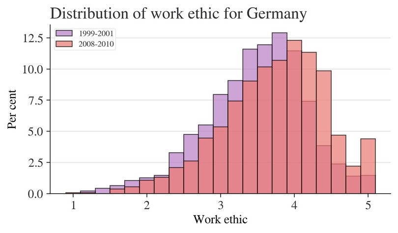
![Distribution of work ethic scores for Germany.]()
Figure 8.2 Distribution of work ethic scores for Germany.
- We will use line charts to make a similar comparison for life satisfaction (
A170) over time. Using data for countries that are present in Waves 1 to 4:
- Create a table showing the average life satisfaction, by wave (column variable) and by country (row variable).
- Plot a line chart with wave number (1 to 4) on the horizontal axis and the average life satisfaction on the vertical axis.
- From your results in 2(a) and (b), how has the distribution of life satisfaction changed over time? What other information about the distribution of life satisfaction could we use to supplement these results?
- Choose one or two countries and research events that could explain the observed changes in average life satisfaction over time shown in 2(a) and (b).
Python walk-through 8.7 Plotting multiple lines on a chart
Calculate average life satisfaction, by wave and country
Before we can plot the line charts, we have to calculate the average life satisfaction for each country in each wave.
In Python walk-through 8.5, we produced summary tables, grouped by country and employment status. We will copy this process, but now we only require mean values. Countries that do not report the life satisfaction variable for all waves will have an average life satisfaction of ‘NA’. Since each country is represented by a row in the summary table, we use the
rowwiseandna.omitfunctions to drop any countries that do not have a value for the average life satisfaction for all four waves.avg_life_sat = ( lifesat_data.groupby(["S002EVS", "S003"])["A170"] # Groupby wave and country .mean() # Take the mean of life satisfaction .unstack() .T.dropna( # One row per country, one wave per column how="any", axis="index" ) # Drop any rows with missing observations ) avg_life_sat
S002EVS 1981–1984 1990–1993 1999–2001 2008–2010 S003 Belgium 7.373659 7.600515 7.417261 7.628444 Denmark 8.208083 8.168627 8.312646 8.408106 France 6.707666 6.770642 6.983779 7.053691 Germany 7.219167 7.028605 7.431564 6.773619 Iceland 8.046307 8.010145 8.076202 8.072072 Ireland 7.815372 7.87663 8.20844 7.823413 Italy 6.651618 7.298985 7.182841 7.398402 Netherlands 7.750459 7.769076 7.827736 7.9904 Northern Ireland 7.659164 7.884868 8.0672 7.81877 Spain 6.59554 7.154639 6.974359 7.288546 Sweden 8.029834 7.991525 7.62406 7.678934 Create a line chart for average life satisfaction
As the data is already in the format suitable for
matplotlib(composed as a matrix), we can almost usedataframe.plotdirectly. But as we want to make a few tweaks and add a few extra details, we need to also create an overall axis (ax) and pass that to the dataframe plotting function (dataframe.plot(ax=ax), afterfig, ax = plt.suplots()).The other settings do minor adjustments to the chart, like setting the y-label (
ax.set_ylabel) and add a legendax.legendthat is outside of the graphed areabbox_to_anchor=(1, 1).fig, ax = plt.subplots() avg_life_sat.T.plot(ax=ax) ax.set_title("Life satisfaction across countries and survey waves", loc="left") ax.legend(bbox_to_anchor=(1, 1)) ax.set_xlabel("Survey wave") ax.set_ylabel("Mean") plt.show()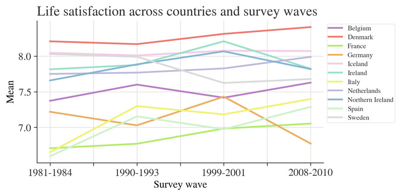
![Line chart of average life satisfaction across countries and survey waves.]()
Figure 8.3 Line chart of average life satisfaction across countries and survey waves.
- correlation coefficient
- A numerical measure, ranging between 1 and −1, of how closely associated two variables are—whether they tend to rise and fall together, or move in opposite directions. A positive coefficient indicates that when one variable takes a high (low) value, the other tends to be high (low) too, and a negative coefficient indicates that when one variable is high the other is likely to be low. A value of 1 or −1 indicates that knowing the value of one of the variables would allow you to perfectly predict the value of the other. A value of 0 indicates that knowing one of the variables provides no information about the value of the other.
After describing patterns in our main variables over time, we will use correlation coefficients and scatter plots to look at the relationship between these variables and the other variables in our dataset.
- Using the Wave 4 data:
- Create a table as shown in Figure 8.4 and calculate the required correlation coefficients. For employment status and gender, you will need to create new variables: full-time employment should be equal to 1 if full-time employed and 0 if unemployed, and treated as missing data (left as a blank cell) otherwise. Gender should be 0 if male and 1 if female.
| Variable | Life satisfaction | Work ethic |
|---|---|---|
| Age | ||
| Education | ||
| Full-time employment | ||
| Gender | ||
| Self-reported health | ||
| Income | ||
| Number of children | ||
| Relative income | ||
| Life satisfaction | 1 | |
| Work ethic | 1 |
Figure 8.4 Correlation between life satisfaction, work ethic and other variables, Wave 4.
- Interpret the coefficients, paying close attention to how the variables are coded. (For example, you could comment on the absolute magnitude and sign of the coefficients). Explain whether the relationships implied by the coefficients are what you expected (for example, would you expect life satisfaction to increase or decrease with health, income, and so forth.)
Python walk-through 8.8 Creating dummy variables and calculating correlation coefficients
To obtain the correlation coefficients between variables, we have to make sure that all variables are numeric. However, the data on gender and employment status is coded using text, so we need to create two new variables (
genderandemployment). (We choose to create a new variable rather than overwrite the original variable so that even if we make a mistake, the raw data is still preserved.)We can use the
np.wherefunction to make the value of the variable conditional on whether a logical statement (such asx["X001"] == "Male") is satisfied or not. As shown below, we can nestnp.wherestatements to create more complex conditions, which is useful if the variable contains more than two values. (An alternative method is to create a categorical column using.astype("category")and then use.cat.codeto turn discrete variables into numbers.)We used two
np.wherestatements for the unemployment variable ("X028") so that the new variable will take the value 1 for full-time employed, 0 for unemployed, and ‘NA’ if neither condition is satisfied.The first step is to ensure that all of the variables we’d like,
"X003","X025A_num","employment","gender","A009","X047D","X011_01","inc_percentile","A170","work_ethic", are numeric. We can check this for the variables we already have with.info():lifesat_data.info()<class 'pandas.core.frame.DataFrame'> Index: 129515 entries, 0 to 164995 Data columns (total 21 columns): # Column Non-Null Count Dtype --- ------ -------------- ----- 0 S002EVS 129515 non-null object 1 S003 129515 non-null object 2 S006 129515 non-null int64 3 A009 105426 non-null Int32 4 A170 129515 non-null Int32 5 C036 73912 non-null Int32 6 C037 73912 non-null Int32 7 C038 73912 non-null Int32 8 C039 73912 non-null Int32 9 C041 73912 non-null Int32 10 X001 129515 non-null object 11 X003 129515 non-null object 12 X007 129515 non-null object 13 X011_01 49823 non-null Int32 14 X025A 49823 non-null object 15 X028 129515 non-null object 16 X047D 73912 non-null float64 17 X025A_num 49823 non-null Int32 18 X025A_sch 49823 non-null object 19 work_ethic 73912 non-null object 20 inc_percentile 73912 non-null float64 dtypes: Int32(9), float64(2), int64(1), object(9) memory usage: 18.4+ MBWe need to convert one variable (
X003) fromobjecttofloat.lifesat_data["X003"] = lifesat_data["X003"].astype("float")# Note that the columns employment and gender don't exist yet; we'll create them in the next line of code cols_to_select = [ "X003", "X025A_num", "employment", "gender", "A009", "X047D", "X011_01", "inc_percentile", "A170", "work_ethic", ] corr_matrix = ( lifesat_data.loc[lifesat_data["S002EVS"] == "2008-2010", :] .assign( gender=lambda x: np.where(x["X001"] == "Male", 0, 1), employment=lambda x: np.where( x["X028"] == "Full time", 1, np.where(x["X028"] == "Unemployed", 0, np.nan) ), ) .loc[:, cols_to_select] .corr() )We used the
assignmethod here. It can get confusing when performing operations on columns and rows because there are several different methods you can use:assign,apply,transform, andagg.agg,apply, andtransformare all methods that you use after agroupbyoperation.Here’s a quick guide on when to use each of the three that follow a
groupby:
- Use
.aggwhen you’re using agroupby, but you want your groups to become the new index (rows).- Use
.transformwhen you’re using agroupby, but you want to retain your original index.- Use
.applywhen you’re using agroupby, but you want to perform operations that will leave neither the original index nor an index of groups.Let’s see examples of all three on some dummy data. First, let’s create some dummy data:
len_s = 1000
prng = np.random.default_rng(42)  # prng=probabilistic random number generator
s = pd.Series(
    index=pd.date_range("2000-01-01", periods=len_s, name="date", freq="D"),
    data=prng.integers(-10, 10, size=len_s),
)
s.head()
date 2000-01-01 -9 2000-01-02 5 2000-01-03 3 2000-01-04 -2 2000-01-05 -2 Freq: D, dtype: int64Now let’s see the result of using each kind of the three:
print("\n`.agg` following `.groupby`: groups provide index")
print(s.groupby(s.index.to_period("M")).agg("skew").head())
print("\n`.transform` following `.groupby`: retain original index")
print(s.groupby(s.index.to_period("M")).transform("skew").head())
print("\n`.apply` following `.groupby`: index entries can be new")
print(s.groupby(s.index.to_period("M")).apply(lambda x: x[x > 0].cumsum()).head())
`.agg` following `.groupby`: groups provide index date 2000-01 -0.364739 2000-02 -0.186137 2000-03 0.017442 2000-04 -0.298289 2000-05 -0.140669 Freq: M, dtype: float64 `.transform` following `.groupby`: retain original index date 2000-01-01 -0.364739 2000-01-02 -0.364739 2000-01-03 -0.364739 2000-01-04 -0.364739 2000-01-05 -0.364739 Freq: D, dtype: float64 `.apply` following `.groupby`: index entries can be new date date 2000-01 2000-01-02 5 2000-01-03 8 2000-01-06 15 2000-01-08 18 2000-01-12 27 dtype: int64
assign, meanwhile, is used when you want to add new columns to a dataframe in place. Its sister function is the pure assignment by creating a new column directly (using=). Let’s see the effect of both of these on the dummy data:# Makes a dataframe rather than just a series s = pd.DataFrame(s, columns=["number"]) # Creating data directly s["new_column_directly"] = 10 s.head()
number new_column_directly date 2000-01-01 −9 10 2000-01-02 5 10 2000-01-03 3 10 2000-01-04 −2 10 2000-01-05 −2 10 And now using
assign:# Creating data using assign s = s.assign(new_column_indirectly=11) s.head()
number new_column_directly new_column_indirectly date 2000-01-01 −9 10 11 2000-01-02 5 10 11 2000-01-03 3 10 11 2000-01-04 −2 10 11 2000-01-05 −2 10 11 Let’s return to the correlation matrix we created:
# Only interested in two columns, so select those
corr_matrix.loc[:, ["A170", "work_ethic"]]
A170 work_ethic X003 −0.082205 0.133333 X025A_num 0.093639 −0.145356 employment 0.183873 −0.027108 gender −0.021055 −0.047816 A009 0.375603 −0.073209 X047D 0.235425 −0.152270 X011_01 −0.017294 0.089255 inc_percentile 0.295930 −0.186799 A170 1.000000 −0.033525 work_ethic −0.033525 1.000000
Next we will look at the relationship between employment status and life satisfaction, and investigate the paper’s hypothesis that this relationship varies with a country’s average work ethic.
- Using the data from Wave 4, carry out the following:
- Create a table showing the average life satisfaction according to employment status (showing the full-time employed, retired, and unemployed categories only) with country (
S003) as the row variable, and employment status (X028) as the column variable. Comment on any differences in average life satisfaction between these three groups, and whether social norms is a plausible explanation for these differences.
- Use the table from Question 4(a) to calculate the difference in average life satisfaction across categories of individuals (full-time employed minus unemployed, and full-time employed minus retired).
- Make a separate scatterplot for each of these differences in life satisfaction, with average work ethic on the horizontal axis and difference in life satisfaction on the vertical axis.
- For each difference (employed versus unemployed, employed versus retired), calculate and interpret the correlation coefficient between average work ethic and difference in life satisfaction.
Python walk-through 8.9 Calculating group means
Calculate average life satisfaction and differences in average life satisfaction
We can achieve the tasks in Question 4(a) and (b) in one go using an approach similar to that used in Python walk-through 8.5, although now we are interested in calculating the average life satisfaction by country and employment type. Once we have tabulated these means, we can compute the difference in the average values. We will create two new variables:
D1for the difference between the average life satisfaction for full-time employed and unemployed, andD2for the difference in average life satisfaction for full-time employed and retired individuals.# Set the employment types that we wish to report employment_list = ["Full time", "Retired", "Unemployed"] df_employment = ( lifesat_data.loc[ (lifesat_data["S002EVS"] == "2008-2010") & (lifesat_data["X028"].isin(employment_list)), # Row selection :, # Col selection—all columns ] # Select wave 4 and these specific emp types .groupby(["S003", "X028"]) # Group by country and employment type .mean(numeric_only=True)[ "A170" ] # Mean value of life satisfaction by country and employment .unstack() # Reshape to one row per country (country is inner layer) .assign( # Create the differences in means D1=lambda x: x["Full-time"] - x["Unemployed"], D2=lambda x: x["Full-time"] - x["Retired"], ) ) df_employment.round(2)
X028 Full time Retired Unemployed D1 D2 S003 Albania 6.63 5.81 6.07 0.57 0.83 Armenia 6.04 4.85 5.46 0.58 1.18 Austria 7.44 7.74 6.07 1.36 −0.31 Belarus 6.1 5.62 5.61 0.49 0.48 Belgium 7.72 7.83 6.37 1.35 −0.12 Bosnia Herzegovina 7.33 7.01 6.77 0.56 0.33 Bulgaria 6.18 4.97 4.69 1.48 1.2 Croatia 7.31 6.48 7.17 0.14 0.83 Cyprus 7.38 7.03 6.56 0.82 0.35 Czech Republic 7.3 6.89 6.07 1.24 0.42 Denmark 8.54 8.21 7.2 1.34 0.34 Estonia 6.93 6.25 4.97 1.95 0.67 Finland 7.82 8.02 5.77 2.05 −0.2 France 7.2 6.97 6.24 0.96 0.23 Georgia 6.12 4.69 5.42 0.7 1.43 Germany 7.26 6.85 4.61 2.65 0.41 Great Britain 7.53 7.93 6.03 1.51 −0.4 Greece 7.15 6.62 5.98 1.17 0.53 Hungary 6.65 5.89 4.86 1.79 0.76 Iceland 8.2 8.45 7.23 0.97 −0.24 Ireland 7.9 7.83 7.18 0.71 0.07 Italy 7.43 7.44 6.6 0.83 −0.01 Kosovo 6.3 6.04 6.78 −0.49 0.26 Latvia 6.52 5.93 5.31 1.21 0.59 Lithuania 6.59 5.63 4.53 2.06 0.96 Luxembourg 7.87 8.24 5.5 2.37 −0.37 Macedonia 7.19 6.67 6.61 0.58 0.52 Malta 7.7 7.76 5.95 1.75 −0.06 Moldova 7.12 5.98 6.07 1.05 1.14 Montenegro 7.63 7.22 7.47 0.16 0.42 Netherlands 8.04 7.95 7.0 1.04 0.09 Northern Cyprus 6.74 6.44 5.64 1.1 0.29 Northern Ireland 7.68 7.77 7.54 0.14 −0.09 Norway 8.19 8.26 8.0 0.19 −0.07 Poland 7.46 6.57 7.06 0.4 0.89 Portugal 6.84 5.88 5.44 1.4 0.96 Romania 7.14 6.57 7.41 −0.27 0.56 Russian Federation 6.86 5.7 6.4 0.46 1.16 Serbia 7.17 6.67 6.73 0.44 0.5 Slovakia 7.47 6.71 6.12 1.35 0.76 Slovenia 7.83 7.13 6.76 1.07 0.7 Spain 7.34 7.21 7.19 0.15 0.13 Sweden 7.88 8.17 6.52 1.36 −0.3 Switzerland 8.04 8.12 5.76 2.28 −0.08 Turkey 6.5 6.61 5.76 0.74 −0.11 Ukraine 6.34 5.44 4.95 1.4 0.9 Make a scatterplot sorted according to work ethic
To plot the differences ordered by the average work ethic, we first need to get all data from Wave 4 (using
.loc), summarize thework_ethicvariable by country (groupbythen take themean), and store the results in a temporary dataframe (df_work_ethic).df_work_ethic = ( lifesat_data.loc[ (lifesat_data["S002EVS"] == "2008-2010"), ["S003", "work_ethic"] ] # Select wave 4 and two columns only .groupby(["S003"]) # Group by country .mean() # Mean value of work_ethic by country ) df_work_ethic.head().round(2)
work_ethic S003 Albania 3.922667 Armenia 3.885621 Austria 3.722533 Belarus 3.619563 Belgium 3.313477 We can now combine the mean
work_ethicdata with the table containing the difference in means, using an ‘inner join’ (how="inner") to match the data correctly by country. Then we make a scatterplot usingmatplotlib. This process can be repeated for the difference in means between full-time employed and retired individuals by changingy = D1toy = D2in the function we create for plotting.df_emp_ethic_comb = pd.merge(df_employment, df_work_ethic, on=["S003"], how="inner") fig, ax = plt.subplots() ax.scatter(df_emp_ethic_comb["work_ethic"], df_emp_ethic_comb["D1"]) ax.set_ylabel("Difference") ax.set_xlabel("Work ethic") ax.set_title( "Difference in wellbeing between people who are employed full-time and people who are unemployed versus work ethic", size=14, ) ax.set_ylim(0, None) plt.show()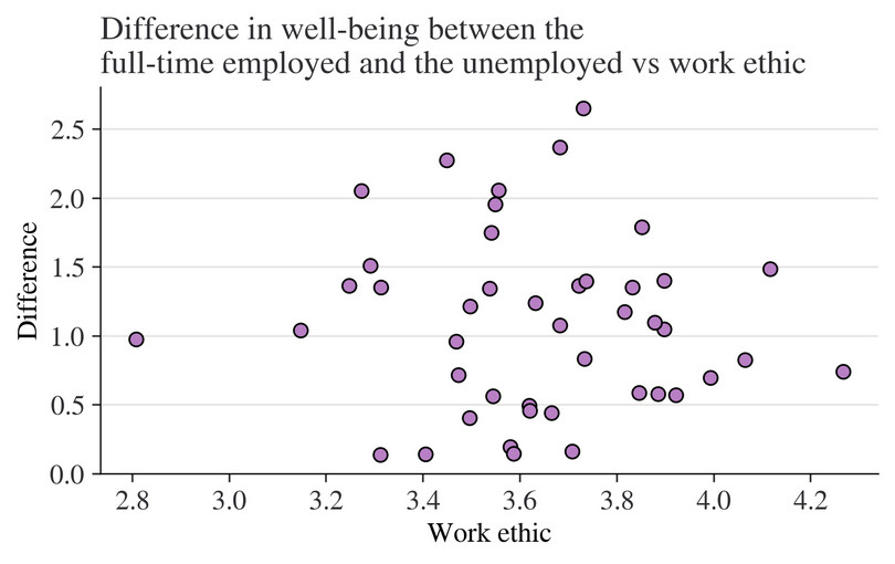
![Difference in life satisfaction (wellbeing) between people who are employed full-time and people who are unemployed versus average work ethic.]()
Figure 8.5 Difference in life satisfaction (wellbeing) between people who are employed full-time and people who are unemployed versus average work ethic.
To calculate correlation coefficients, use the
corrfunction applied to a dataframe. You can see that the correlation between average work ethic and difference in life satisfaction is quite weak for people who are employed versus people who are unemployed, but moderate and positive for people who are employed versus people who are retired.df_emp_ethic_comb.corr().loc[["D1", "D2"], ["work_ethic"]]
work_ethic D1 −0.157565 D2 0.484261
So far, we have described the data using tables and charts, but have not made any statements about whether what we observe is consistent with an assumption that work ethic has no bearing on differences in life satisfaction between different subgroups. In the next part, we will assess the relationship between employment status and life satisfaction and assess whether the observed data lead us to reject the above assumption.
Part 8.3 Confidence intervals for difference in the mean
Note
You will need to have done Questions 1–5 in Part 8.1 before doing this part. Part 8.2 is not necessary, but is helpful to get an idea of what the data looks like.
Learning objectives for this part
- Calculate and interpret confidence intervals for the difference in means between two groups.
The aim of this project was to look at the empirical relationship between employment and life satisfaction.
When we calculate differences between groups, we collect evidence which may or may not support a hypothesis that life satisfaction is identical between different subgroups. Economists often call this testing for statistical significance. In Part 6.2 of Empirical Project 6, we constructed 95% confidence intervals for means, and used a rule of thumb to assess our hypothesis that the two groups considered were identical (at the population level) in the variable of interest. Now we will learn how to construct confidence intervals for the difference in two means, which allows us to make such a judgment on the basis of a single confidence interval.
Remember that the width of a confidence interval depends on the standard deviation and number of observations. (Read Part 6.2 of Empirical Project 6 to understand why.) When making a confidence interval for a sample mean (such as the mean life satisfaction of people who are unemployed), we use the sample standard deviation and number of observations in that sample (unemployed people) to obtain the standard error of the sample mean.
\[\text{Standard error of sample mean (SE)} = \frac{\text{SD of sample data}}{\sqrt{\text{number of observations } (n)}}\]When we look at the difference in means (such as life satisfaction of employed people minus that of unemployed people), we are using data from two groups (the unemployed and the employed) to make one confidence interval. To calculate the standard error for the difference in means, we use the standard errors (SE) of each group:
\[\text{SE (difference in means)} = \sqrt{(\text{SE of group 1})^2 + (\text{SE of group 2})^2}\]This formula requires the two groups of data to be independent, meaning that the data from one group is not related, paired, or matched with data from the other group. This assumption is reasonable for the life satisfaction data we are using. However, if the two groups of data are not independent, for example if the same people generated both groups of data (as in the public goods experiments of Empirical Project 2), then we cannot use this formula.
Once we have the new standard error and number of observations, we can calculate the width of the confidence interval (that is, the distance from the mean to one end of the interval) as before. The width of the confidence interval tells us how precisely the difference in means was estimated, and this precision tells us how compatible the sample data is with the hypothesis that there is no difference between the population means. If the value 0 falls outside the 95% confidence interval, this implies that the data is unlikely to have been sampled from a population with equal population means. For example, if the estimated difference is positive, and the 95% confidence interval is not wide enough to include 0, we can be reasonably confident that the true difference is positive too. In other words, it tells us that the p-value for the difference we have found is less than 0.05, so we would be very unlikely to find such a big difference if the population means were in fact identical.
In Figure 8.6, for Great Britain, we can be reasonably confident that the true difference in average life satisfaction between people who are full-time employed and people who are unemployed is positive. However, for Spain, we do not have strong evidence of a real difference in mean life satisfaction.
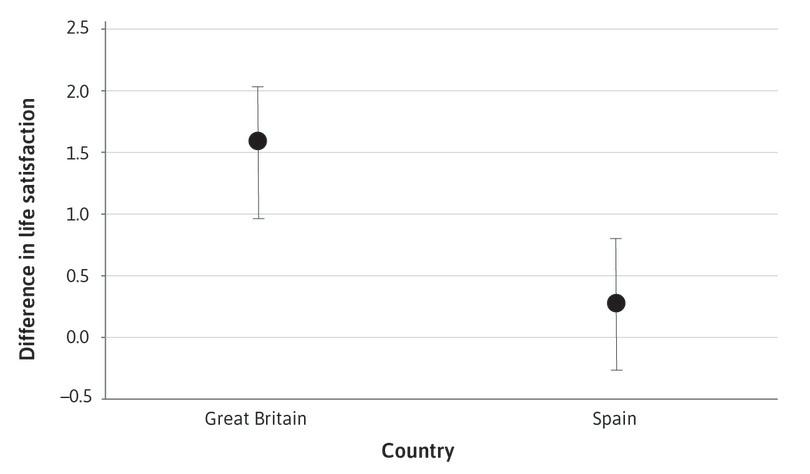
Figure 8.6 95% confidence intervals for the average difference in life satisfaction (people who are full-time employed minus people who are unemployed) in Great Britain and Spain.
- We will apply this method to make confidence intervals for differences in life satisfaction. Choose three countries: one with an average work ethic in the top third of scores, one in the middle third, and one in the lower third. (See Python walk-through 6.3 for help on calculating confidence intervals and adding them to a chart.)
-
In Question 4 of Part 8.2, you computed the average life satisfaction score by country and employment type (using Wave 4 data). Repeat this procedure to obtain the standard error for the means for each of your chosen countries.
Create a table for these countries, showing the average life satisfaction score, standard deviation of life satisfaction, and number of observations, with country (
S003) as the row variable, and employment status (full-time employed, retired, and unemployed only) as the column variable.
- Use your table from Question 1(a) to calculate the difference in means across categories of individuals (full-time employed minus unemployed, and full-time employed minus retired), the standard deviation of these differences, the number of observations, and the confidence interval.
- Use Python’s
ttestfunction to determine the 95% confidence interval width of the difference in means and compare your results with Question 1(b).
- Plot a column chart for your chosen countries showing the difference in life satisfaction across categories of individuals (employed versus unemployed and employed versus retired) on the vertical axis, and country on the horizontal axis (sorted according to low, medium, and high work ethic). Add the confidence intervals from Question 1(c) to your chart.
- Interpret your findings from Question 1(d), commenting on the size of the observed differences in means, and the precision of your estimates.
Python walk-through 8.10 Calculating confidence intervals and adding error bars
We will use Turkey, Spain, and Great Britain as example countries in the top, middle, and bottom third of work ethic scores, respectively.
In the tasks in Questions 1(a) and (b), we will obtain the means, standard errors, and 95% confidence intervals step-by-step, then for Question 1(c), we show how to use a shortcut to obtain confidence intervals from a single function.
Calculate confidence intervals manually
We obtained the difference in means in Python walk-through 8.9 (
D1andD2), so now we can calculate the standard error of the means for each country of interest. We’ll do this calculation manually, using the formula.country_list = ["Turkey", "Spain", "Great Britain"] df_emp_se = ( lifesat_data.loc[ (lifesat_data["S002EVS"] == "2008-2010") & (lifesat_data["X028"].isin(employment_list)) & (lifesat_data["S003"].isin(country_list)), :, ] # Select the relevant employment types, countries, and wave 4 .groupby(["S003", "X028"]) # Groupby country and employment type .apply(lambda x: x["A170"].std() / np.sqrt(x["A170"].count())) # .std(ddof=0)["A170"] # Find the standard dev of life satisfaction .unstack() # Put the employment types along the columns .assign( # Calculate the standard errors of the differences D1_SE=lambda x: (x["Full time"].pow(2) + x["Unemployed"].pow(2)).pow(1 / 2), D2_SE=lambda x: (x["Full time"].pow(2) + x["Retired"].pow(2)).pow(1 / 2), ) ) df_emp_se.round(2)
X028 Full time Retired Unemployed D1_SE D2_SE S003 Great
Britain0.10 0.12 0.25 0.27 0.15 Spain 0.09 0.14 0.25 0.27 0.17 Turkey 0.14 0.18 0.18 0.23 0.23 We can now combine the standard errors with the difference in means, and compute the 95% confidence interval width.
df_emp_subset = (
    df_employment.loc[df_employment.index.isin(country_list), ["D1", "D2"]]
    .join(df_emp_se.loc[:, ["D1_SE", "D2_SE"]], how="inner")
    .assign(CI_1=lambda x: 1.96 * x["D1_SE"], CI_2=lambda x: 1.96 * x["D2_SE"])
)

df_emp_subset.round(3)
X028 D1 D2 D1_SE D2_SE CI_1 CI_2 S003 Great
Britain1.507 −0.398 0.267 0.154 0.524 0.302 Spain 0.145 0.127 0.265 0.168 0.520 0.330 Turkey 0.737 −0.107 0.229 0.231 0.449 0.452 We now have a table containing the difference in means, the standard error of the difference in means, and the confidence intervals for each of the two differences. (Recall that
D1is the difference between the average life satisfaction for full-time employed and unemployed, andD2is the difference in average life satisfaction for people who are full-time employed and people who are retired.)Calculate confidence intervals using a t-test function
We could obtain the confidence intervals directly by using the
ttestfunction from thepingouinpackage. We already imported it at the start of this project, but if you didn’t already, runimport pingouin as pg.First, we need to prepare the data in two groups. In the following example, we calculate the difference in average life satisfaction for full-time employed and unemployed people in Turkey, but the process can be repeated for the difference between full-time employed and retired people by changing the code appropriately (also for your other two chosen countries).
We start by selecting the data for full-time and unemployed people in Turkey, and storing it in two separate temporary matrices (arrays of rows and columns) called
turkey_fullandturkey_unemployed, respectively, which is the format needed for the t-test function.# Create a Boolean that's true for wave 4, Turkey, and full-time full_boolean = ( (lifesat_data["S002EVS"] == "2008-2010") & (lifesat_data["S003"] == "Turkey") & (lifesat_data["X028"] == "Full time") ) turkey_full = ( lifesat_data.loc[full_boolean, ["A170"]] # Select the life satisfaction data .astype("double") # Ensure this is a floating point number .values # Grab the values--this is needed for the t-test ) # Do the same for the unemployed unem_boolean = ( (lifesat_data["S002EVS"] == "2008-2010") & (lifesat_data["S003"] == "Turkey") & (lifesat_data["X028"] == "Unemployed") ) turkey_unemployed = lifesat_data.loc[unem_boolean, ["A170"]].astype("double").valuesIn the code above, for full time employment, we created a Boolean row filter based on three different columns using:
lifesat_data["S002EVS"] == "2008-2010" & lifesat_data["S003"] == "Turkey" & lifesat_data["X028"] == "Full time"and put this result into
.locusing the.loc[rows, columns]syntax..locisn’t the only way to select rows to operate on, though: an alternative is to use.queryand pass it a string (some text) that asks for particular column values. This is easiest to demonstrate with an example:turkey_full = ( lifesat_data # Select wave 4, Turkey, and full time .query("S002EVS == '2008-2010' and S003 == 'Turkey' and X028 == 'Full time'") .loc[:, ["A170"]] # Select the life satisfaction data .astype("double") # Ensure this is a floating point number .values # Grab the values--this is needed for the t-test )You can see we still use a
.locafter the query line, but only to select columns. (We select all rows from the previous step using:.)Sometimes
.querycan be shorter or clearer to write than a conditional statement; it varies depending on the case. (Try and see if you can write the equivalent query for the unemployed.) It’s useful to know both but, if in doubt, simply use.loc.Let’s return to the task. We can use the
ttestfunction from thepingouinpackage on the two newly created vectors. The default confidence interval level is 95% and can be changed via theconfidence=keyword argument. Note that theravelfunction turns an array like[[1], [5], [0]]into an array of the form[1, 5, 0].ttest = pg.ttest(turkey_full.ravel(), turkey_unemployed.ravel()).round(3) ttest
T dof alternative p-val CI95% cohen-d BF10 power T-test 3.218 575.096 two-sided 0.001 [0.29, 1.19] 0.26 13.551 0.901 We can then calculate the difference in means by finding the midpoint of the interval (
ttest["CI95%"].iloc[0].mean()is 0.74), which should be the same as the figures obtained in Question 1(b) (df.employment\[3, 2\]is 0.7374582).Add error bars to the column charts
We can now use these confidence intervals (and widths) to add error bars to our column charts. To do so, we use the
geom_errorbaroption, and specify the lower and upper levels of the confidence interval for theyminandymaxoptions respectively. In this case, it is easier to use the results from Questions 1(a) and (b), as we already have the values for the difference in means and the CI width stored as variables.fig, ax = plt.subplots() ax.bar(df_emp_subset.index, df_emp_subset["D1"], yerr=df_emp_subset["CI_1"]) ax.set_xlabel("Country", labelpad=10) ax.set_xlabel("Country") ax.set_title("Difference in wellbeing (full-time versus unemployed)") plt.show()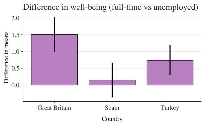
![Difference in life satisfaction (wellbeing) between people who are full-time employed and people who are unemployed.]()
Figure 8.7 Difference in life satisfaction (wellbeing) between people who are full-time employed and people who are unemployed.
Again, this can be repeated for the difference in life satisfaction between full-time employed and retired. Remember to change
df_emp_subset["D1"]todf_emp_subset["D2"], and change the error bars correspondingly.
- The method we used to compare life satisfaction relied on making comparisons between people with different employment statuses, but a person’s employment status is not entirely random. We cannot therefore make causal statements such as ‘being unemployed causes life satisfaction to decrease’. Describe how we could use the following methods to assess better the effect of being unemployed on life satisfaction, and make some statements about causality:
- a natural experiment
- panel data (data on the same individuals, taken at different points in time).
