9. Credit-excluded households in a developing country Working in Python
Download the code
To download the code chunks used in this project, right-click on the download link and select ‘Save Link As…’. You’ll need to save the code download to your working directory, and open it in Python.
Don’t forget to also download the data into your working directory by following the steps in this project.
Getting started in Python
Visit the ‘Getting started in Python’ page for help and advice on setting up a Python session to work with. Remember, you can run any page from this book as a notebook by downloading the relevant file from this repository and running it on your own computer. Alternatively, you can run pages online in your browser over at Binder .
Preliminary settings
Let’s import the packages we’ll need and also configure the settings we want:
import pandas as pd
import matplotlib.pyplot as plt
import numpy as np
from pathlib import Path
import pingouin as pg
from lets_plot import *

LetsPlot.setup_html(no_js=True)
Part 9.1 Households that did not get a loan
Learning objectives for this part
- Identify credit-constrained and credit-excluded households using survey information.
- Create dummy (indicator) variables.
- Compare characteristics of successful borrowers, discouraged borrowers, credit-constrained households, and credit-excluded households.
- Explain why selection bias is an important issue.
The Ethiopian Socioeconomic Survey (ESS) data was collected in 2013–14 from a nationally representative sample of households. Households were asked about topics such as their housing conditions, assets, and access to credit.
Download the ESS data and survey questionnaire:
- Download the ESS data. The Excel file contains three tabs (‘Data dictionary’, ‘All households’, and ‘Got loan’). Read the ‘Data dictionary’ tab and make sure you know what each variable represents. For Part 9.1, we will use the data from the ‘All households’ tab. The ‘Got loan’ data will be used in Part 9.2.
- For the documentation, go to the data download site. Click on the ‘Documentation’ tab in the middle of the page.
- Under the heading ‘Questionnaires’, download the PDF file called ‘2013–2014 Ethiopian Socioeconomic Survey, Household Questionnaire’ by clicking the ‘Download’ button on the right-hand side of the page. You may find it helpful to refer to Section 14 of the questionnaire for the exact questions asked about credit and saving.
Python walk-through 9.1 Importing data into Python
Ensure that the Excel file you downloaded is in a sub-directory of your working directory called ‘data’.
Before importing the data, open it in Excel to look at its structure. You can see there are three tabs: ‘Data dictionary’, ‘All households’, and ‘Got loan’. We will import them into separate dataframes (
data_dict,all_hh, andgot_l, respectively). We import the ‘Data dictionary’ so that we do not have to return to the Excel spreadsheet.Also note that there are many empty cells, which is how missing data is coded in Excel (but not in Python). In the
pd.read_excelfunction, the default setting is that empty cells are read asNA, so we don’t need to specify this. Note thatpandasmay warn you about an ‘unknown extension’: an Excel file is actually a bundle of files tied up to look like one file, andpandasdoesn’t recognize one of the files in the bundle. Still, this warning won’t prevent us from importing the data we need from the worksheets.data_dict = pd.read_excel( Path("data/doing-economics-working-in-excel-project-9-datafile.xlsx"), sheet_name="Data dictionary", ) all_hh = pd.read_excel( Path("data/doing-economics-working-in-excel-project-9-datafile.xlsx"), sheet_name="All households", ) got_l = pd.read_excel( Path("data/doing-economics-working-in-excel-project-9-datafile.xlsx"), sheet_name="Got loan", )Now let’s look at the variable types
all_hhandgot_lusing the.info()method.all_hh.info()<class 'pandas.core.frame.DataFrame'> RangeIndex: 5262 entries, 0 to 5261 Data columns (total 19 columns): # Column Non-Null Count Dtype --- ------ -------------- ----- 0 household_id2 5262 non-null int64 1 got_loan 5250 non-null object 2 rural 5262 non-null object 3 hhsize 5260 non-null float64 4 region 5262 non-null object 5 gender 5261 non-null object 6 age 5253 non-null float64 7 young_children 5262 non-null int64 8 working_age_adults 5262 non-null int64 9 max_education 5262 non-null float64 10 number_assets 5262 non-null int64 11 loan_rejected 5259 non-null object 12 rejection_source1 226 non-null object 13 rejection_source2 48 non-null object 14 loan_purpose 221 non-null object 15 loan_purpose_other 52 non-null object 16 did_not_apply 5223 non-null object 17 reason_not_apply1 3592 non-null object 18 reason_not_apply2 2015 non-null object dtypes: float64(3), int64(4), object(12) memory usage: 781.2+ KBgot_l.info()<class 'pandas.core.frame.DataFrame'> RangeIndex: 1480 entries, 0 to 1479 Data columns (total 21 columns): # Column Non-Null Count Dtype --- ------ -------------- ----- 0 household_id2 1480 non-null int64 1 got_loan 1470 non-null category 2 rural 1480 non-null category 3 hhsize 1478 non-null float64 4 region 1480 non-null category 5 gender 1480 non-null category 6 age 1479 non-null float64 7 young_children 1480 non-null int64 8 working_age_adults 1480 non-null int64 9 max_education 1480 non-null float64 10 number_assets 1480 non-null int64 11 borrowed_from 1470 non-null category 12 borrowed_from_other 147 non-null category 13 loan_purpose 1444 non-null category 14 loan_startmonth 1476 non-null category 15 loan_startyear 1477 non-null float64 16 loan_repaid 1478 non-null category 17 loan_endmonth 946 non-null category 18 loan_endyear 946 non-null float64 19 loan_amount 1479 non-null float64 20 loan_interest 1445 non-null float64 dtypes: category(10), float64(7), int64(4) memory usage: 145.1 KBIt is important to ensure that all variables we expect to be numerical (numbers) have either
intorfloatlisted as their ‘Dtype’, and in this case, they are. You can see that there are many variables that are coded asobjectvariables because they are text (for examplegenderorregion), but since we can use these variables to group data by category, we will use.astype("category")to change them into categorical variables for later use.Instead of converting each object variable to a factor variable individually, we can use the
select_dtypesmethod to find all columns that are currently of typeobjectand then convert those columns specifically.cols = all_hh.select_dtypes("object").columns all_hh[cols] = all_hh[cols].astype("category") cols = got_l.select_dtypes("object").columns got_l[cols] = got_l[cols].astype("category")Making use of
.info()will now show you that the remaining object columns have been ‘recast’ to be of data type ‘category’.
- The data is already in a format clean enough to use, so we will begin by summarizing the information in the ‘All households’ tab, starting with region and household characteristics.
- Create a table showing the proportion of households that lived in each region and area type, with
regionas the row variable andruralas the column variable. (For help on creating tables, see Python walk-through 3.3.)
- Use the
Gendervariable to find what percentage of household heads were female.
- Create an appropriate summary table for the variables
hhsize,gender,age,young_children,working_age_adults,max_education, andnumber_assets. (You may find it helpful to refer to Python walk-through 2.7 in Empirical Project 2 for one possible format to use.)
- Write a short paragraph describing the information in your tables for 1(c).
Python walk-through 9.2 Creating summary tables
To get the proportions of households in each region living in large towns, small towns, or rural areas (encoded in the variable
rural), we use thepd.crosstabfunction to create a cross-tabulation. Without any further options,pd.crosstabwould produce counts of households in the respective regions and area types. However, we can pass a keyword argument,normalize, to turn the counts into proportions by rows or columns.In the code below, we use
normalize="index"to ensure that each row sums to one. We also use.round(3) to specify the number of decimal places that are saved in the output data frame.Remember that if you ever want to know more about a function, you can hover over it in Visual Studio Code to see its options, including the keyword arguments it takes. Or you can run
help(function-name), wherefunction-nameis the name of the function you need more information about.stab_one = pd.crosstab(all_hh["region"], all_hh["rural"], normalize="index").round(3) stab_one
rural Large town (urban) Rural Small town (urban) region Addis Ababa 1.000 0.000 0.000 Afar 0.096 0.757 0.147 Amhara 0.218 0.669 0.113 Benshagul Gumuz 0.000 0.904 0.096 Diredwa 0.468 0.532 0.000 Gambelia 0.115 0.800 0.085 Harari 0.273 0.727 0.000 Oromia 0.283 0.607 0.110 SNNP 0.183 0.727 0.090 Somalie 0.155 0.755 0.090 Tigray 0.367 0.563 0.070 Let’s use a similar approach to calculate the percentage of households with women as head of the family (encoded in the variable
gender).stab_two = all_hh["gender"].value_counts(normalize=True).round(3) stab_twogender Male 0.696 Female 0.304 Name: proportion, dtype: float64As shown, 30.4% of households have a head of the family who is a woman.
We need to provide summary statistics for a range of variables. Most of these variables are numeric variables, but one,
gender, is a categorical variable. We can distinguish these types using the.select_dtypesmethod.There are a few different ways to get summary statistics on a data frame.
pandashas a built-in method called.describe, which produces different information depending on whether the given columns are numeric or not. Here it is running on just numeric columns:all_hh.select_dtypes("number").describe().round(2)
household_id2 hhsize age young_children working_age_adults max_education number_assets count 5.262000e+03 5,260.00 5,253.00 5,262.00 5,262.00 5,262.00 5,262.00 mean 5.759796e+16 4.58 44.18 1.89 2.58 7.53 14.90 std 3.938921e+16 2.40 15.61 1.71 1.52 7.28 17.23 min 1.010109e+16 1.00 3.00 0.00 0.00 0.00 0.00 25% 3.051509e+16 3.00 32.00 0.00 2.00 2.00 5.00 50% 4.150101e+16 4.00 42.00 2.00 2.00 6.00 9.00 75% 7.110409e+16 6.00 55.00 3.00 3.00 10.00 18.00 max 1.501021e+17 16.00 99.00 10.00 10.00 30.00 203.00 If we use it on a categorical variable,
gender, we get information relevant to that type of data:all_hh["gender"].describe()count 5261 unique 2 top Male freq 3662 Name: gender, dtype: objectA more powerful way to summarize a dataframe is provided by a package called
skimpy(which you can install by runningpip install skimpyin the command line). Here is skimpy’sskimfunction applied toall_hh:from skimpy import skim skim(all_hh)╭──────────────────────────────────────────────── skimpy summary ─────────────────────────────────────────────────╮ │ Data Summary Data Types Categories │ │ ┏━━━━━━━━━━━━━━━━━━━┳━━━━━━━━┓ ┏━━━━━━━━━━━━━┳━━━━━━━┓ ┏━━━━━━━━━━━━━━━━━━━━━━━┓ │ │ ┃ dataframe ┃ Values ┃ ┃ Column Type ┃ Count ┃ ┃ Categorical Variables ┃ │ │ ┡━━━━━━━━━━━━━━━━━━━╇━━━━━━━━┩ ┡━━━━━━━━━━━━━╇━━━━━━━┩ ┡━━━━━━━━━━━━━━━━━━━━━━━┩ │ │ │ Number of rows │ 5262 │ │ category │ 12 │ │ got_loan │ │ │ │ Number of columns │ 19 │ │ int64 │ 4 │ │ rural │ │ │ └───────────────────┴────────┘ │ float64 │ 3 │ │ region │ │ │ └─────────────┴───────┘ │ gender │ │ │ │ loan_rejected │ │ │ │ rejection_source1 │ │ │ │ rejection_source2 │ │ │ │ loan_purpose │ │ │ │ loan_purpose_other │ │ │ │ did_not_apply │ │ │ │ reason_not_apply1 │ │ │ │ reason_not_apply2 │ │ │ └───────────────────────┘ │ │ number │ │ ┏━━━━━━━━━━━━━━━━━━━┳━━━━┳━━━━━━┳━━━━━━━━━┳━━━━━━━━━┳━━━━━━━┳━━━━━━━━━┳━━━━━━━━━┳━━━━━━━━━┳━━━━━━━━━┳━━━━━━━━┓ │ │ ┃ column_name ┃ NA ┃ NA % ┃ mean ┃ sd ┃ p0 ┃ p25 ┃ p50 ┃ p75 ┃ p100 ┃ hist ┃ │ │ ┡━━━━━━━━━━━━━━━━━━━╇━━━━╇━━━━━━╇━━━━━━━━━╇━━━━━━━━━╇━━━━━━━╇━━━━━━━━━╇━━━━━━━━━╇━━━━━━━━━╇━━━━━━━━━╇━━━━━━━━┩ │ │ │ household_id2 │ 0 │ 0 │ 5.8e+16 │ 3.9e+16 │ 1e+16 │ 3.1e+16 │ 4.2e+16 │ 7.1e+16 │ 1.5e+17 │ ▇▆▆ ▁▃ │ │ │ │ hhsize │ 2 │ 0.04 │ 4.6 │ 2.4 │ 1 │ 3 │ 4 │ 6 │ 16 │ ▇▇▆▁ │ │ │ │ age │ 9 │ 0.17 │ 44 │ 16 │ 3 │ 32 │ 42 │ 55 │ 99 │ ▇▇▅▂ │ │ │ │ young_children │ 0 │ 0 │ 1.9 │ 1.7 │ 0 │ 0 │ 2 │ 3 │ 10 │ ▇▆▂▁ │ │ │ │ working_age_adult │ 0 │ 0 │ 2.6 │ 1.5 │ 0 │ 2 │ 2 │ 3 │ 10 │ ▃▇▂▁ │ │ │ │ s │ │ │ │ │ │ │ │ │ │ │ │ │ │ max_education │ 0 │ 0 │ 7.5 │ 7.3 │ 0 │ 2 │ 6 │ 10 │ 30 │ ▇▆▃▁ ▁ │ │ │ │ number_assets │ 0 │ 0 │ 15 │ 17 │ 0 │ 5 │ 9 │ 18 │ 200 │ ▇▁ │ │ │ └───────────────────┴────┴──────┴─────────┴─────────┴───────┴─────────┴─────────┴─────────┴─────────┴────────┘ │ │ category │ │ ┏━━━━━━━━━━━━━━━━━━━━━━━━━━━━━━━━━━━━━━━━━━┳━━━━━━━━━━━━━┳━━━━━━━━━━━━━━━┳━━━━━━━━━━━━━━━━━━┳━━━━━━━━━━━━━━━━┓ │ │ ┃ column_name ┃ NA ┃ NA % ┃ ordered ┃ unique ┃ │ │ ┡━━━━━━━━━━━━━━━━━━━━━━━━━━━━━━━━━━━━━━━━━━╇━━━━━━━━━━━━━╇━━━━━━━━━━━━━━━╇━━━━━━━━━━━━━━━━━━╇━━━━━━━━━━━━━━━━┩ │ │ │ got_loan │ 12 │ 0.23 │ False │ 3 │ │ │ │ rural │ 0 │ 0 │ False │ 3 │ │ │ │ region │ 0 │ 0 │ False │ 11 │ │ │ │ gender │ 1 │ 0.02 │ False │ 3 │ │ │ │ loan_rejected │ 3 │ 0.06 │ False │ 3 │ │ │ │ rejection_source1 │ 5036 │ 95.71 │ False │ 10 │ │ │ │ rejection_source2 │ 5214 │ 99.09 │ False │ 9 │ │ │ │ loan_purpose │ 5041 │ 95.8 │ False │ 9 │ │ │ │ loan_purpose_other │ 5210 │ 99.01 │ False │ 15 │ │ │ │ did_not_apply │ 39 │ 0.74 │ False │ 3 │ │ │ │ reason_not_apply1 │ 1670 │ 31.74 │ False │ 11 │ │ │ │ reason_not_apply2 │ 3247 │ 61.71 │ False │ 11 │ │ │ └──────────────────────────────────────────┴─────────────┴───────────────┴──────────────────┴────────────────┘ │ ╰────────────────────────────────────────────────────── End ──────────────────────────────────────────────────────╯Now we can see lots of information on both the categorical and numeric data types!
Now that we have an idea of what our data looks like, we will move on to identifying households that are potentially excluded from the credit market or are credit constrained. The former are households that find it impossible to borrow, and the latter are households that can only borrow on unfavourable terms (see Section 9.10 of Economy, Society, and Public Policy).
The variables in our dataset that are related to this issue are did_not_apply and loan_rejected. Later we will also look at the responses given in the variables reason_not_apply1 and reason_not_apply2.
- Using the ‘All households’ dataset:
- Create a frequency table with
did_not_applyas the row variable andloan_rejectedas the column variable. Include all ‘NA’ as a separate row.
- Looking at these two variables, explain why some observations should be excluded and remove them from the dataset. Also remove all households with missing information for one or more of these variables. Of the non-excluded observations, what percentage of households applied for a loan over the past 12 months? Of those households, what percentage were successful?
- For the resulting categories in the frequency table, explain whether the households in that category can be described as credit constrained, credit excluded, or both.
Python walk-through 9.3 Making frequency tables for loan applications and outcomes
The easiest way to make a frequency table is to use the
pd.crosstabfunction. Note that we use thedropna=Falseoption (and ‘All’ minus the sum of ‘No’ and ‘Yes’ gives the number of ‘NA’s), and themargins=True optionto give those totals.stab_three = pd.crosstab( all_hh["did_not_apply"], all_hh["loan_rejected"], dropna=False, margins=True ) stab_three
loan_rejected No Yes All did_not_apply Applied 1,363 201 1,565 Did not apply 3,632 24 3,658 All 5,032 227 5,262 Now we will do some data cleaning and re-examine the table. We:
- exclude the households that indicated that they did not apply for a loan, but also indicated that they were refused a loan. This step results in excluding more than 10% of households that indicated that they were refused a loan, because their answer is nonsensical. We will use the
~operator, which means ‘not’ (when applied to the logic that follows).- We will also remove all observations that have missing data for any of these two questions, by using the implicit default value of
dropna=True.all_hh_c = all_hh.loc[ ~( (all_hh["loan_rejected"] == "Yes") & (all_hh["did_not_apply"] == "Did not apply") ), :, ].copy() stab_four = pd.crosstab( all_hh_c["did_not_apply"], all_hh_c["loan_rejected"], margins=True, normalize="all" ).round(3) stab_four
loan_rejected No Yes All did_not_apply Applied 0.262 0.039 0.301 Did not apply 0.699 0.000 0.699 All 0.961 0.039 1.000 In the code above, we used the classic syntax for accessing rows and columns,
.loc[rows, columns]. Because we wanted all columns, we used:. We also used.copy()to create a new set of data calledall_hh_c. Without this step, any modifications we made toall_hh_cwould also be applied toall_hh.
To create operational categories to use throughout this project, we will label households as either:
- ‘successful’: households that applied for a loan and were given the loan
- ‘denied’: households that applied but were not given the loan
- ‘did not apply’: households that did not apply for a loan.
You should note that the ‘denied’ households are only a subset of the credit-excluded households, as there will be households that are credit excluded and do not even apply for a loan. One could, for instance, reason that households who answered ‘Inadequate Collateral’ or ‘Do Not Know Any Lender’ are also likely to be credit excluded.
- Using the subset of data from Question 2(b):
- Create a new variable called
HH_statuswith the above categories.
- Create a new variable
discouraged_borrowerthat takes the value 1 if the household did not apply for a loan because it believed that it would not receive a loan (answered ‘Believe Would Be Refused’ inreason_not_apply1orreason_not_apply2). How many households (and what percentage) are discouraged borrowers? (Note: This is a fairly narrow definition of ‘discouraged’ and one could easily argue that other criteria should also be considered under this label.)
Note that arguably other answers are also indicative of being credit constrained, so the criteria we use is definitely only a subset of all households that are credit constrained. For example, one could include households that have been denied a loan, and it is also likely that some households that have been granted a loan are in fact credit constrained.
- Create a new variable
credit_constrainedthat takes the value 1 (or yes) for households that gave a reason for not applying other than ‘NA’, ‘Other’, or ‘Have Adequate Farm’ in either of the two questionsreason_not_apply1orreason_not_apply2, and 0 otherwise. For example, a household that answers ‘Have Adequate Farm’ inreason_not_apply1and ‘Do Not Know Any Lender’ would not be classified as credit constrained. How many households (and what percentage) are credit constrained?
- Create a frequency table showing the most important reason for not applying for a loan, and another showing the second most important reason for not applying. What were the most common reasons for not applying?
Python walk-through 9.4 Creating variables to classify households
Let’s first create the
hh_statusvariable. We set the values ofhh_statusto"not applied", then use logical indexing to change all entries where households applied for a loan (all_hh_c["did_not_apply"] == "Applied") and were accepted (all_hh_c["loan_rejected"] == "No") to"successful", and change all entries where households who were denied (all_hh_c["loan_rejected"] == "Yes") to"denied".# This is the default category and creates the new column all_hh_c["hh_status"] = "not applied" all_hh_c.loc[ (all_hh_c["did_not_apply"] == "Applied") & (all_hh_c["loan_rejected"] == "No"), "hh_status", ] = "successful" all_hh_c.loc[ (all_hh_c["did_not_apply"] == "Applied") & (all_hh_c["loan_rejected"] == "Yes"), "hh_status", ] = "denied" # Change from a string variable to a categorical variable all_hh_c["hh_status"] = all_hh_c["hh_status"].astype("category")Let’s have a look at the frequencies of the different outcomes:
all_hh_c["hh_status"].value_counts()hh_status not applied 3674 successful 1363 denied 201 Name: count, dtype: int64Now we will use the same steps to make the
discouraged_borrowervariable.# This is the default category and creates the new column all_hh_c["discouraged_borrower"] = "No" all_hh_c.loc[ (all_hh_c["reason_not_apply1"] == "Believe Would Be Refused"), "discouraged_borrower", ] = "Yes" all_hh_c.loc[ (all_hh_c["reason_not_apply2"] == "Believe Would Be Refused"), "discouraged_borrower", ] = "Yes" # Change from a string variable to a categorical variable all_hh_c["discouraged_borrower"] = all_hh_c["discouraged_borrower"].astype("category") all_hh_c["discouraged_borrower"].value_counts()discouraged_borrower No 4649 Yes 589 Name: count, dtype: int64To make the
credit_constrainedvariable, we use the.cat.categoriesproperty to check all the possible answers to thereason_not_apply1variable. We store these answers in the objectsel_ans. (To convert from an index, a special type ofpandasobject, to a simple Python list, we put the expression on the right-hand side within alist(..).)sel_ans = list(all_hh_c["reason_not_apply1"].cat.categories) sel_ans['Believe Would Be Refused', 'Do Not Know Any Lender', 'Do Not Like To Be In Debt', 'Fear Not Be Able To Pay', 'Have Adequate Farm', 'Inadequate Collateral', 'No Farm Or Business', 'Other (Specify)', 'Too Expensive', 'Too Much Trouble']Of these reasons, only reasons 4 (‘Have Adequate Farm’) and 7 (‘Other’) do not lead to a conclusion that a household is credit constrained, so we remove them from
sel_ans. Note that this numbering starts from 0.sel_ans.remove("Have Adequate Farm") sel_ans.remove("Other (Specify)") sel_ans['Believe Would Be Refused', 'Do Not Know Any Lender', 'Do Not Like To Be In Debt', 'Fear Not Be Able To Pay', 'Inadequate Collateral', 'No Farm or Business', 'Too Expensive', 'Too Much Trouble']Households that did not provide any reasons are classified as not credit constrained. We’ll take this as our default category and use it to create the column.
all_hh_c["credit_constrained"] = "No"

all_hh_c.loc[all_hh_c["reason_not_apply1"].isin(sel_ans), "credit_constrained"] = "Yes"
all_hh_c.loc[all_hh_c["reason_not_apply2"].isin(sel_ans), "credit_constrained"] = "Yes"

# Turn `credit_constrained` into a categorical variable
all_hh_c["credit_constrained"] = all_hh_c["credit_constrained"].astype("category")
all_hh_c["credit_constrained"].value_counts()
credit_constrained Yes 3020 No 2218 Name: count, dtype: int64The use of
.isinin the selection criterion is a very useful programming technique that you can use to select data according to a list of variables. In this case,sel_anscontains all the answers that we associate with a credit constrained household.
all_hh_c["reason_not_apply1"].isin(sel_ans)gives an outcome ofTrueif the variable taken by an entry in the columnreason_not_apply1is one of the values insel_ans. In that case, it sets the value ofcredit_constrainedto ‘Yes’ for those observations.stab_four = pd.crosstab( all_hh_c["credit_constrained"], all_hh_c["discouraged_borrower"], margins=True, normalize="all", ).round(3) stab_four
discouraged_borrower No Yes All credit_constrained No 0.423 0.000 0.423 Yes 0.464 0.112 0.577 All 0.888 0.112 1.000 Let’s look at the frequencies of the different reasons to not apply (
reason_not_apply1andreason_not_apply2), in descending order.all_hh_c["reason_not_apply1"].value_counts(normalize=True).round(3)reason_not_apply1 Do Not Like To Be In Debt 0.190 Have Adequate Farm 0.185 Fear Not Be Able To Pay 0.170 Believe Would Be Refused 0.116 No Farm Or Business 0.101 Do Not Know Any Lender 0.068 Too Expensive 0.050 Inadequate Collateral 0.046 Other (Specify) 0.041 Too Much Trouble 0.033 Name: proportion, dtype: float64all_hh_c["reason_not_apply2"].value_counts(normalize=True).round(3)reason_not_apply2 Fear Not Be Able To Pay 0.276 Do Not Like To Be In Debt 0.244 Inadequate Collateral 0.087 Believe Would Be Refused 0.086 Too Expensive 0.067 Do Not Know Any Lender 0.063 Too Much Trouble 0.061 Have Adequate Farm 0.050 No Farm Or Business 0.039 Other (Specify) 0.024 Name: proportion, dtype: float64
We will now analyse the stated reasons for wanting a loan, comparing those households that were successful (HH_status equal to ‘successful’) with those that were not successful (HH_status equal to ‘denied’).
- For both groups, create one table showing the proportion of households for each loan purpose. You will realise that in the ‘All households’ dataset, the reason for all ‘successful’ loans is ‘Other’. For that reason, you should use the ‘Got loan’ dataset to retrieve the reasons for loan information for successful loans. Was the purpose of loans for denied and successful borrowers similar? (Hint: It may help to think about the broad categories of spending on consumption and investment.)
Python walk-through 9.5 Making frequency tables to compare proportions
Some of the data is in the
all_hhdataset, while the rest is in thegot_ldataset, both of which we imported in Python walk-through 9.1. We will combine that information into one new dataset calledloan_data, which we then use to produce the table.sel_all_hh_c = all_hh_c.loc[all_hh_c["hh_status"].isin(["successful", "denied"])] pd.crosstab( sel_all_hh_c["loan_purpose"], sel_all_hh_c["hh_status"], margins=True, dropna=False ).round(3)
hh_status denied not applied successful All loan_purpose 10 3 0 0 3 Business Start-Up Capital 51 0 0 51 Expanding Business 27 0 1 28 Other (Specify) 50 0 0 50 Purchase Agricultural Inputs For Food Crop 41 0 0 41 Purchase House/Lease Land 6 0 0 6 Purchase Inputs For Other Crops 12 0 0 12 Purchase Non-Farm Inputs 5 0 0 5 All 201 0 1,363 1,564 This table reveals a particular feature of the data: it doesn’t contain as much useful information as we’d like! Most successful loans actually have ‘NA’ in the box for loan purpose (except one, which has ‘Expanding Business’). The cross-tab above shows us that there were 1,363 successful loans but only one with a purpose.
There is more useful information on loan purpose in the
got_ldata, so we will extract theloan_purposevariable for unsuccessful households from theall_hh_cdataset, and the equivalent information for successful loaners from thegot_ldataset.# Select unsuccessful households from all_hh_c loan_no = all_hh_c.loc[all_hh_c["hh_status"] == "denied", ["loan_purpose", "hh_status"]] # Select loan purpose for successful households from gotL loan_yes = got_l.loc[got_l["got_loan"] == "Yes", ["loan_purpose"]] loan_yes["hh_status"] = "successful" # combine the data through concatenation loan_data = pd.concat([loan_yes, loan_no]) # let's look at the values pd.crosstab( loan_data["loan_purpose"], loan_data["hh_status"], normalize="columns" ).round(3)
hh_status denied successful loan_purpose 10 0.015 0.000 Business Start-Up Capital 0.262 0.154 Expanding Business 0.138 0.081 For Consumption And Personal Expenses 0.000 0.201 Other (Specify) 0.256 0.027 Purchase Agricultural Inputs For Food Crop 0.210 0.300 Purchase House/Lease Land 0.031 0.023 Purchase Inputs For Other Crops 0.062 0.098 Purchase Non-Farm Inputs 0.026 0.115
- Using the information in the ‘All households’ and ‘Got loan’ tab, for ‘successful’ and ‘denied’ households:
- Create a table as shown in Figure 9.1 to compare the averages of the specified household characteristics.
| Household characteristic | Successful | Denied |
|---|---|---|
| Age of household head | ||
| Highest education in household | ||
| Number of assets | ||
| Household size | ||
| Number of young children | ||
| Number of working-age adults |
Figure 9.1 Characteristics of successful and denied borrowers.
- conditional mean
- An average of a variable, taken over a subgroup of observations that satisfy certain conditions, rather than all observations.
- For each characteristic, explain how it may affect a household’s ability to get a loan (ceteris paribus).
- Looking at your table from Question 5(a), discuss whether you see this pattern in the data. (For example, are successful borrowers older/younger on average than denied borrowers?)
- Now try conditioning on the variable
ruralorregionand discuss how (if at all) your results change.
Python walk-through 9.6 Calculating differences in household characteristics
Here we show how to use the
meanfunction to get average characteristics conditional on"hh_status".# Show the number of observations in each category all_hh_c["hh_status"].value_counts()hh_status not applied 3674 successful 1363 denied 201 Name: count, dtype: int64Now let’s look at mean household size conditional on credit status:
all_hh_c.groupby("hh_status").mean(numeric_only=True)["hhsize"].round(2)hh_status denied 4.82 not applied 4.46 successful 4.87 Name: hhsize, dtype: float64What about the mean
max_educationof household head by credit status?all_hh_c.groupby("hh_status").mean(numeric_only=True)["max_education"].round(2)hh_status denied 8.00 not applied 7.61 successful 7.26 Name: max_education, dtype: float64As before, we can use cross-tabs to see the number of observations in each category:
pd.crosstab(
    all_hh_c["rural"],
    all_hh_c["hh_status"],
).round(3)
hh_status denied not applied successful rural Large town (urban) 56 1,096 332 Rural 128 2,272 903 Small town (urban) 17 306 128 To get even more breakdowns, you can add more variables to the
groupby.Let’s see an example with mean household size by the other variables,
ruraland credit status.all_hh_c.groupby(["hh_status", "rural"]).mean(numeric_only=True)["hhsize"].round(2)hh_status rural denied Large town (urban) 3.57 Rural 5.47 Small town (urban) 4.06 not applied Large town (urban) 3.44 Rural 4.98 Small town (urban) 4.27 successful Large town (urban) 3.84 Rural 5.35 Small town (urban) 4.12 Name: hhsize, dtype: float64Or we could make a table showing the number of working-age adults by the
ruraland credit variables:all_hh_c.groupby(["hh_status", "rural"]).mean(numeric_only=True)[ "working_age_adults" ].round(2)hh_status rural denied Large town (urban) 2.36 Rural 2.88 Small town (urban) 3.18 not applied Large town (urban) 2.30 Rural 2.58 Small town (urban) 2.75 successful Large town (urban) 2.42 Rural 2.91 Small town (urban) 2.54 Name: working_age_adults, dtype: float64
- Using Figure 9.1, without conditioning on
ruralorregion:
- Calculate the difference in means (‘successful’ borrowers minus ‘denied’ borrowers).
- Calculate the 95% confidence interval for the difference in means between the two subgroups (‘successful’ minus ‘denied’). (See Part 8.3 of Empirical Project 8 for help on how to do this.)
- Plot a column chart showing the differences on the vertical axis (sorted from smallest to largest), and household characteristics on the horizontal axis. Add the confidence intervals from Question 6(b) to the chart.
- Interpret your findings.
Python walk-through 9.7 Calculating confidence intervals and adding them to a chart
To repeat the same set of calculations for a list of variables, first we create a list of these variables (called
sel_var).sel_var = [ "age", "max_education", "number_assets", "hhsize", "young_children", "working_age_adults", ]Now we use the
agevariable as an example, removing the ‘did not apply’ ("not applied") entries.stats_5 = ( all_hh_c.groupby("hh_status")["age"] .agg({"mean", "count", "std"}) .drop("not applied") .round(2) ) stats_5
mean count std hh_status denied 41.21 201 12.85 successful 43.37 1,361 14.27 Now we use the
ttestfunction from thepingouinpackage to calculate the difference between the successful group (sel_success) and the denied borrowers (sel_denied).import pingouin as pg # Select the age variable (aka sel_var[0]) for successful and # denied borrowers sel_success = all_hh_c.loc[all_hh_c["hh_status"] == "successful", sel_var[0]] sel_denied = all_hh_c.loc[all_hh_c["hh_status"] == "denied", sel_var[0]] # do the t-test. Default confidence is 0.95, but include it here to be explicit pg.ttest(x=sel_success, y=sel_denied, confidence=0.95).round(3)
T dof alternative p-val CI95% cohen-d BF10 power T-test 2.186 278.073 two-sided 0.03 [0.21, 4.09] 0.153 0.872 0.525 The output of this test indicates whether the ages of the two groups are statistically different. (Here, they are.)
We will now do this for all variables of interest and save the difference in means and the confidence interval values in a dataframe, so we can plot this information.
To make this easier, we’ll write a function that:
- takes the name of the variable of interest as function
- selects successful and unsuccessful applicants, and performs a t-test on that variable (like we already did for age)
- returns the answers (the difference in means and the upper and lower confidence limits) in a format useful for populating a dataframe of results.
We will create an empty dataframe to populate with this information and then run the whole task in a loop.
def get_ttest_and_mean_for_variable(dataframe_variable, selected_variable):
    """Given a dataframe with loan statuses encoded by a "hh_status" column
    with values of "successful" and "denied", and columns that have other
    relevant characteristics, this function returns the mean difference between
    the successful and denied households according to the characteristic given
    by the 'selected_variable'.

    Args:
        dataframe_name (pandas dataframe): Data containing loan outcomes.
        selected_variable (string): Name of other characteristic.

    Returns:
        list (floats): Mean difference, low limit conf int, high limit conf int
    """
    # Select the variable for successful and
    # denied borrowers
    sel_success = dataframe_variable.loc[
        dataframe_variable["hh_status"] == "successful", selected_variable
    ]
    sel_denied = dataframe_variable.loc[
        dataframe_variable["hh_status"] == "denied", selected_variable
    ]

    # Do the t-test. Default confidence is 0.95, but include it here to be explicit
    pg.ttest(x=sel_success, y=sel_denied, confidence=0.95).round(3)

    mean_difference = sel_success.mean() - sel_denied.mean()
    mean_low, mean_high = (
        pg.ttest(x=sel_success, y=sel_denied, confidence=0.95)
        .round(3)["CI95%"]
        .explode()
        .to_list()
    )
    return mean_difference, mean_low, mean_high

# create an empty dataframe for the results
data_to_plot = pd.DataFrame()

# Now we can loop through the variables
for this_variable in sel_var:
    mean_diff, low, high = get_ttest_and_mean_for_variable(all_hh_c, this_variable)
    temp_data = pd.DataFrame.from_dict(
        {
            "var_name": this_variable,
            "mean_difference": mean_diff,
            "conf_low": low,
            "conf_high": high,
        },
        orient="index",
    ).T
    data_to_plot = pd.concat([temp_data, data_to_plot], axis=0)

# give different rows different index numbers (dropping old index)
data_to_plot = data_to_plot.reset_index(drop=True)
data_to_plot.head()
var_name mean_difference conf_low conf_high 0 working_age_adults −0.003468 −0.22 0.21 1 young_children −0.135106 −0.4 0.13 2 hhsize 0.046946 −0.3 0.4 3 number_assets 1.421393 −1.13 3.97 4 max_education −0.73457 −1.89 0.42 Now we can plot the chart using
lets_plot.# Rename the rows in `var_name` so the y-axis labels will look neater data_to_plot = data_to_plot.replace( { "age": "Age", "max_education": "Max education", "number_assets": "Number of assets", "hhsize": "Household size", "young_children": "Young children", "working_age_adults": "Working-age adults" } ) ( ggplot( data_to_plot.reset_index(), aes( x="var_name", y="mean_difference", fill="var_name", ), ) + geom_bar(stat="identity", show_legend=False, color="black", alpha=0.6) + geom_errorbar( aes(ymin="conf_low", ymax="conf_high", color="var_name"), size=2, show_legend=False, ) + labs( y="Mean difference", x="Variable name" ) + coord_flip() )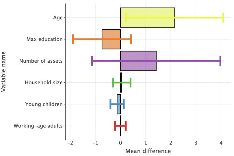
![]()
Figure 9.2 Bar chart showing difference in household characteristics for successful and denied borrowers.
- Using the information in the ‘All households’ dataset:
- Create a table similar to Figure 9.1, but with additional columns for discouraged borrowers and credit-constrained households.
- Compare the means across the four groups and discuss any similarities/differences you observe (you do not need to do any formal calculations).
Python walk-through 9.8 Calculating conditional means
We are interested in the means of a range of variables for different subgroups. Two subgroups are mutually exclusive (
hh_status == "successful"andhh_status == "denied"), while the others (credit_constrained == "yes"anddiscouraged_borrower == "yes") are partially overlapping subgroups of the data. Our strategy is to create a temporary dataframe (sel_all_hh_c) that only contains the relevant observations and the relevant variables. Then we can calculate the required means using the built-in.meanmethod ofpandas.# variables we are interested in sel_var = [ "age", "max_education", "number_assets", "hhsize", "young_children", "working_age_adults", ] sel_all_hh_c = all_hh_c.loc[all_hh_c["hh_status"] == "successful", sel_var] print(f"Successful, n = {len(sel_all_hh_c)}")Successful, n = 1363Now we get the means of each column:
sel_all_hh_c.mean(axis="index").round(2)age 43.37 max_education 7.26 number_assets 15.88 hhsize 4.87 young_children 2.09 working_age_adults 2.75 dtype: float64We can perform the same operation with
denied:sel_all_hh_c = all_hh_c.loc[all_hh_c["hh_status"] == "denied", sel_var] print(f"Denied, n = {len(sel_all_hh_c)}")Denied, n = 201You can re-calculate the conditional means based on this dimension, too:
sel_all_hh_c.mean(axis="index").round(2)age 41.21 max_education 8.00 number_assets 14.46 hhsize 4.82 young_children 2.22 working_age_adults 2.76 dtype: float64You can use similar methods to look at discouraged and credit constrained households.
An article by the Institute for Work and Health explains selection bias in more detail, and why it is a problem encountered by all areas of research.
- selection bias
- An issue that occurs when the sample or data observed is not representative of the population of interest. For example, individuals with certain characteristics may be more likely to be part of the sample observed (such as students being more likely than CEOs to participate in computer lab experiments).
A study on access to loans in Ethiopia looked at the relationship between loan amount and household characteristics. When doing so, they needed to account for selection bias, because we only observe positive loan amounts for successful borrowers. If we only had data for successful borrowers, then our sample would not be representative of the population of interest (all households), so we would have to interpret our results with caution. In our case, we have information about all households, so we can compare observable characteristics to see whether successful borrowers are similar to other households.
- Think of another example where there might be selection bias, in other words, where the data we observe is not representative of the population of interest.
Part 9.2 Households that got a loan
Learning objectives for this part
- Analyse the characteristics of loans obtained by successful borrowers.
For households that successfully got a loan, we will look at:
- the purpose of the loan
- the duration of the loan(s)
- the loan amount and interest rate charged
- who the household borrowed from.
We will also see if there are any relationships between these loan characteristics and household characteristics.
Now we will use the variables relating to the loan start and end dates to calculate the duration of the loan. Before using these variables, we need to check that the variable entries make sense. Some of this information could be recorded incorrectly (for example, the year is missing a digit, or the month is a number rather than a word).
- Using the ‘Got loan’ dataset:
- Check the variables
loan_startmonth,loan_startyear,loan_endmonth, andloan_endyear, and replace the entries that are recorded incorrectly with either the correct entry (if possible), or as blank (if not possible to infer the correct entry). (Note: Some entries are recorded as ‘Pagume’, which corresponds to early September in the Ethiopian calendar.)
- To calculate loan duration, combine the month and year variables into one date variable and format them as date variables.
- Some of the dates (months or years) are missing. Calculate the percentage of the data that is missing and explain whether you think missing data is a serious problem.
- Create a new variable containing the loan duration (end date minus start date), which will be measured in days.
- You will notice that some dates were recorded incorrectly, with the start date later than the end date. We could either treat these entries as missing or swap the start and end dates. Create two new variables for loan duration, one with all negative entries recorded as blank, and one with negative entries replaced as positive numbers.
- For this project we will define a long-term loan as lasting more than a year (365 days), which we will use in later questions. For this definition, use the
loan_lengthvariable that converts negative loan lengths to positive ones (see Question 1(e) above). Create an indicator variable calledlong_termthat equals 1 if the loan was long term, and 0 otherwise. What percentage of loans were long term?
Python walk-through 9.9 Data cleaning and summarizing loan characteristics
We start by cleaning up the loan dates. We have information on start month and year as well as end month and year. Let’s look at these in turn. The structure of the dataframe,
got_l.info(), indicates that the start and end year are numeric variables, but the months are factor variables with month names (for example ‘April’).Let’s first look at the years by creating a scatterplot.
(
    ggplot(got_l, aes(x="loan_endyear", y="loan_startyear"))
    + geom_point(size=6)
    + labs(
        title="Loan start and end year", y="Loan start year", x="Loan end year"
    )
    + scale_x_continuous(format="d")
    + scale_y_continuous(format="d")
)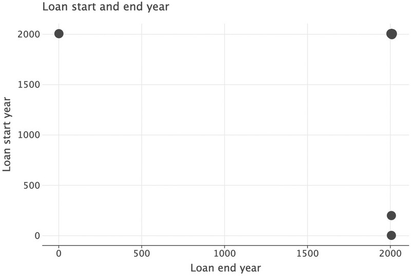
![]()
Figure 9.3 Scatterplot showing loan start and end year.
We can see that there are three observations that have very low start or end year values (less than 500), which does not make sense. We will replace these with
pd.NA, but leave the original data untouched and create a new dataset calledgot_l_c, where the ‘c’ indicates cleaned data.got_l_c = got_l.copy() got_l_c.loc[ (got_l_c["loan_startyear"] < 500) | (got_l_c["loan_endyear"] < 500), ["loan_startyear", "loan_endyear"], ] = pd.NA( ggplot(got_l_c, aes(x="loan_endyear", y="loan_startyear")) + geom_point() + labs( title="Loan start and end year", y="Loan start year", x="Loan end year" ) + scale_x_continuous(format="d") + scale_y_continuous(format="d") )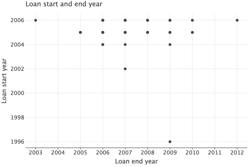
![]()
Figure 9.4 Revised scatterplot showing loan start and end year without outliers.
In the top-left corner, there is a loan with the start year (2006) after the end year (2003). Clearly this data entry is incorrect, so we should remove this observation when analysing loan periods. However, we will wait until we have combined the years with the months as there may be more observations with this issue.
Also, we can only see a small number of points because there are many identical observations (for example, a start year of 2006 and end year of 2006). To see these points you can add
position=position_jitter()to thelets_plotplotting command. Hover your mouse over the function within an integrated development environment to see whatposition_jitter()does.( ggplot(got_l_c, aes(x="loan_endyear", y="loan_startyear")) + geom_point(position=position_jitter()) + labs( title="Loan start and end year", y="Loan start year", x="Loan end year" ) + scale_x_continuous(format="d") + scale_y_continuous(format="d") )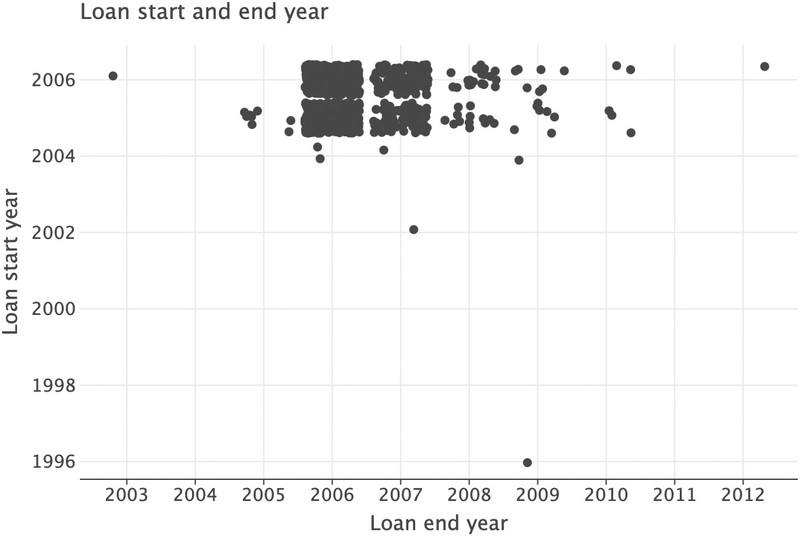
![]()
Figure 9.5 Revised scatterplot of loan start and end year, with jitter added to data points.
Now let’s look at the values in
loan_startmonth. We’ll keep any null (NA) values because we’re interested in missing observations here.got_l_c["loan_startmonth"].value_counts(dropna=False)loan_startmonth January 176 June 156 September 146 February 145 May 141 December 133 July 115 November 115 October 106 April 95 March 85 August 63 NaN 4 Name: count, dtype: int64This data all looks fine apart from the
NaN(not a number) entries; what about the end months?got_l_c["loan_endmonth"].value_counts(dropna=False)loan_endmonth NaN 534 February 170 March 155 April 136 June 94 May 89 August 53 January 52 December 49 October 39 September 37 July 34 November 33 Pagume 5 Name: count, dtype: int64Two things are noteworthy here: there are many
NaNentries, and there is an entry called ‘Pagume’. As described in the task, ‘Pagume’ can be approximated by September. Let’s recode that accordingly, and recode theNaNsto ‘Missing’.got_l_c.loc[got_l_c["loan_endmonth"] == "Pagume", "loan_endmonth"] = "September" for col in ["loan_startmonth", "loan_endmonth"]: # add a 'missing' category got_l_c[col] = got_l_c[col].cat.add_categories("missing") # fill na with 'missing' got_l_c[col] = got_l_c[col].fillna("missing") for col in ["loan_startyear", "loan_endyear"]: # first convert to integer to remove .0 at end # then to string, with missing replacing nans got_l_c[col] = got_l_c[col].astype("Int64").astype("string").fillna("missing")You can check that the end months now have sensible entries for the valid rows.
Let’s now calculate the length of the loan; in other words, the number of days between start and end day.
pandashas very powerful functionality for dates and times. Our first step is to create a new variable that combines months and years together. We can do this by ‘casting’ (using.astype) columns as strings and then usingpd.to_datetime. We have to coerce anyNaNvalues, otherwise we will get an error.Here’s an example (you may get a ‘user warning’ from Python, which you can ignore):
pd.to_datetime(
    got_l_c["loan_startmonth"].astype("str") + "-" + got_l_c["loan_startyear"],
    errors="coerce",
)
0 2004-03-01 1 2006-11-01 2 2006-11-01 3 2005-06-01 4 2005-06-01 ... 1475 2005-08-01 1476 2006-09-01 1477 2006-01-01 1478 2005-07-01 1479 2006-12-01 Length: 1480, dtype: datetime64[ns]Note that it is assumed that we’re counting from the first day of each month.
pd.to_datetimeis converting whatever we feed it to the closest datetime that is similar. A datetime is a special type of variable in computer science: it encodes year, month, day, hours, minutes and seconds. Timing is important, so this variable type is incredibly useful!
pd.to_datetimewill always make a best guess based on what you put in. See what happens if you try putting in a string like ‘15-March-2004’ instead. If you don’t want your date to be at the start of the month, you can ‘add’ the month end on to the date using+ pd.offsets.MonthEnd().Now let’s put the months into the dataframe (using start month as the default):
got_l_c["loan_start_datetime"] = pd.to_datetime(
    got_l_c["loan_startmonth"].astype("str") + "-" + got_l_c["loan_startyear"],
    errors="coerce",
)
got_l_c["loan_end_datetime"] = pd.to_datetime(
    got_l_c["loan_endmonth"].astype("str") + "-" + got_l_c["loan_endyear"],
    errors="coerce",
)
Let’s assess how much missing data we have (as a proportion of the categories we’re interested in):
summary_nans = (
    got_l_c.isna()
    .agg(["sum", "count"])
    .loc[:, ["loan_start_datetime", "loan_end_datetime"]]
    .T
)
summary_nans["pct"] = 100 * summary_nans["sum"] / summary_nans["count"]
summary_nans.round(2)
sum count pct loan_start_datetime 7 1,480 0.47 loan_end_datetime 537 1,480 36.28 So we now have start and end dates in datetime formats. We now compute the difference:
got_l_c["loan_length"] = got_l_c["loan_end_datetime"] - got_l_c["loan_start_datetime"]
got_l_c["loan_length"].head()
0 NaT 1 NaT 2 -153 days 3 273 days 4 245 days Name: loan_length, dtype: timedelta64[ns]Note the following:
- We are missing some loans that didn’t have start or end dates, which have appeared as
NaT(that is, ‘Not a Time’).- Some loan lengths are negative because the recorded end date is before the start date. (It could be that the two dates were switched when the data was entered into the system.)
These data problems are unfortunate but a common feature of real-life empirical work, and you will have to be on the lookout for them!
As required in Question 1, we will create two variants of the
loan_lengthvariable: one where we assign missing values to all observations that have negativeloan_length(loan_length_na), and one where we assume that the problem was the switching of start and end date, so we transform all loan lengths to positive values (loan_length_abs).# Create the missing values version got_l_c["loan_length_na"] = got_l_c["loan_length"].copy() # Set anything less than 0 days to ‘NaT’ got_l_c.loc[got_l_c["loan_length_na"] < pd.Timedelta(0, "d"), "loan_length_na"] = pd.NaT # Create the absolute version got_l_c["loan_length_abs"] = got_l_c["loan_length"].copy() # Set anything less than 0 days to its reverse got_l_c.loc[ got_l_c["loan_length_abs"] < pd.Timedelta(0, "d"), "loan_length_abs" ] = -got_l_c.loc[got_l_c["loan_length_abs"] < pd.Timedelta(0, "d"), "loan_length_abs"]Now we can create the
long_termvariable and look at the number of long-term loans.got_l_c.loc[got_l_c["loan_length_abs"].isna(), "long_term"] = pd.NA got_l_c.loc[got_l_c["loan_length_abs"] > pd.Timedelta(365, "d"), "long_term"] = True got_l_c.loc[got_l_c["loan_length_abs"] < pd.Timedelta(365, "d"), "long_term"] = False got_l_c["long_term"].value_counts(dropna=False)long_term NaN 742 False 523 True 215 Name: count, dtype: int64We therefore have about 23% loans that are long-term (only looking at loans for which we do have date information).
- Using the variables
loan_amountandloan_interest:
- Create summary tables to summarize the distribution of loan amount (mean, standard deviation, maximum, and minimum): one using the loan amount, the other using the total amount to repay (loan amount + interest). Make sure to exclude the one observation previously identified as having an extremely high interest rate. Remember to give your tables meaningful titles. Describe any features of the data that you find interesting.
- As mentioned earlier, the interest rate is a borrowing condition that can vary widely across households. Here we will take the interest rate to be the interest paid as a percentage of the loan amount. Calculate the interest rate for each loan in the data. (Exclude observations where the interest paid is not recorded.)
- Check for extreme values (interest rates that are either very large or zero). You may also want to create a scatterplot (with interest rate on the vertical axis and loan amount on the horizontal axis) to help you identify extreme (atypical) observations. Exclude the observation with the most extreme interest rate from further calculations. What percentage of the loans are zero interest?
- Make summary tables of the mean, maximum, minimum, and quartiles of the loan amount and interest rate, calculating these measures separately for long-term and short-term loans. Compare the distributions of interest rates for short-term and long-term loans.
- Create a table showing the correlation between the interest rate and household characteristics (you may want to refer to Figure 8.4 in Empirical Project 8 for an example). Interpreting the interest rate charged as a measure of default risk (inability to repay), explain whether the relationships implied by the coefficients are what you expected (for example, would you expect interest rates to be higher for households with less assets, more dependents, etc.).
Python walk-through 9.10 Making summary tables and calculating correlations
To make summary tables, we use the
skimfunction from theskimpypackage.from skimpy import skim skim(got_l_c)╭───────────────────────────────────── skimpy summary ──────────────────────────────────────╮ │ Data Summary Data Types Categories │ │ ┏━━━━━━━━━━━━━━━━━━━┳━━━━━━━━┓ ┏━━━━━━━━━━━━━┳━━━━━━━┓ ┏━━━━━━━━━━━━━━━━━━━━━━━┓ │ │ ┃ dataframe ┃ Values ┃ ┃ Column Type ┃ Count ┃ ┃ Categorical Variables ┃ │ │ ┡━━━━━━━━━━━━━━━━━━━╇━━━━━━━━┩ ┡━━━━━━━━━━━━━╇━━━━━━━┩ ┡━━━━━━━━━━━━━━━━━━━━━━━┩ │ │ │ Number of rows │ 1480 │ │ category │ 10 │ │ got_loan │ │ │ │ Number of columns │ 27 │ │ float64 │ 5 │ │ rural │ │ │ └───────────────────┴────────┘ │ int64 │ 4 │ │ region │ │ │ │ timedelta64 │ 3 │ │ gender │ │ │ │ string │ 2 │ │ borrowed_from │ │ │ │ datetime64 │ 2 │ │ borrowed_from_other │ │ │ │ bool │ 1 │ │ loan_purpose │ │ │ └─────────────┴───────┘ │ loan_startmonth │ │ │ │ loan_repaid │ │ │ │ loan_endmonth │ │ │ └───────────────────────┘ │ │ number │ │ ┏━━━━━━━━━━┳━━━━┳━━━━━━┳━━━━━━━━━┳━━━━━━━━━┳━━━━━━━┳━━━━━━━┳━━━━━━━┳━━━━━━━━━━┳━━━━━━━━┓ │ │ ┃ column_n ┃ NA ┃ NA % ┃ mean ┃ sd ┃ p0 ┃ p25 ┃ p75 ┃ p100 ┃ hist ┃ │ │ ┃ ame ┃ ┃ ┃ ┃ ┃ ┃ ┃ ┃ ┃ ┃ │ │ ┡━━━━━━━━━━╇━━━━╇━━━━━━╇━━━━━━━━━╇━━━━━━━━━╇━━━━━━━╇━━━━━━━╇━━━━━━━╇━━━━━━━━━━╇━━━━━━━━┩ │ │ │ househol │ 0 │ 0 │ 4.7e+16 │ 3.5e+16 │ 1e+16 │ 3e+16 │ 7e+16 │ 1.5e+17 │ █▄▄ ▁ │ │ │ │ d_id2 │ │ │ │ │ │ │ │ │ │ │ │ │ hhsize │ 2 │ 0.14 │ 5 │ 2.3 │ 1 │ 3 │ 6 │ 15 │ ▇█▇▃ │ │ │ │ age │ 1 │ 0.07 │ 43 │ 14 │ 4 │ 33 │ 52 │ 99 │ ▆█▄▁ │ │ │ │ young_ch │ 0 │ 0 │ 2.2 │ 1.7 │ 0 │ 1 │ 3 │ 9 │ █▅▇▁▁ │ │ │ │ ildren │ │ │ │ │ │ │ │ │ │ │ │ │ working_ │ 0 │ 0 │ 2.8 │ 1.5 │ 0 │ 2 │ 4 │ 10 │ ▂█▂▁ │ │ │ │ age_adul │ │ │ │ │ │ │ │ │ │ │ │ │ ts │ │ │ │ │ │ │ │ │ │ │ │ │ max_educ │ 0 │ 0 │ 7.1 │ 6.6 │ 0 │ 3 │ 9 │ 30 │ ██▃▁ ▁ │ │ │ │ ation │ │ │ │ │ │ │ │ │ │ │ │ │ number_a │ 0 │ 0 │ 16 │ 19 │ 0 │ 6 │ 19 │ 200 │ █▁ │ │ │ │ ssets │ │ │ │ │ │ │ │ │ │ │ │ │ loan_amo │ 1 │ 0.07 │ 27000 │ 780000 │ 1 │ 400 │ 3500 │ 30000000 │ █ │ │ │ │ unt │ │ │ │ │ │ │ │ │ │ │ │ │ loan_int │ 35 │ 2.36 │ 1800 │ 36000 │ 0 │ 0 │ 400 │ 1300000 │ █ │ │ │ │ erest │ │ │ │ │ │ │ │ │ │ │ │ └──────────┴────┴──────┴─────────┴─────────┴───────┴───────┴───────┴──────────┴────────┘ │ │ category │ │ ┏━━━━━━━━━━━━━━━━━━━━━━━━━━━━━━━━━━┳━━━━━━━━━━┳━━━━━━━━━━━━┳━━━━━━━━━━━━━━┳━━━━━━━━━━━━┓ │ │ ┃ column_name ┃ NA ┃ NA % ┃ ordered ┃ unique ┃ │ │ ┡━━━━━━━━━━━━━━━━━━━━━━━━━━━━━━━━━━╇━━━━━━━━━━╇━━━━━━━━━━━━╇━━━━━━━━━━━━━━╇━━━━━━━━━━━━┩ │ │ │ got_loan │ 10 │ 0.68 │ False │ 3 │ │ │ │ rural │ 0 │ 0 │ False │ 3 │ │ │ │ region │ 0 │ 0 │ False │ 11 │ │ │ │ gender │ 0 │ 0 │ False │ 2 │ │ │ │ borrowed_from │ 10 │ 0.68 │ False │ 11 │ │ │ │ borrowed_from_other │ 1333 │ 90.07 │ False │ 16 │ │ │ │ loan_purpose │ 36 │ 2.43 │ False │ 9 │ │ │ │ loan_startmonth │ 0 │ 0 │ False │ 13 │ │ │ │ loan_repaid │ 2 │ 0.14 │ False │ 3 │ │ │ │ loan_endmonth │ 0 │ 0 │ False │ 13 │ │ │ └──────────────────────────────────┴──────────┴────────────┴──────────────┴────────────┘ │ │ datetime │ │ ┏━━━━━━━━━━━━━━━━━━━━━━━━━━┳━━━━━━┳━━━━━━━━━┳━━━━━━━━━━━━━━┳━━━━━━━━━━━━━━┳━━━━━━━━━━━━┓ │ │ ┃ column_name ┃ NA ┃ NA % ┃ first ┃ last ┃ frequency ┃ │ │ ┡━━━━━━━━━━━━━━━━━━━━━━━━━━╇━━━━━━╇━━━━━━━━━╇━━━━━━━━━━━━━━╇━━━━━━━━━━━━━━╇━━━━━━━━━━━━┩ │ │ │ loan_start_datetime │ 7 │ 0.47 │ 1996-09-01 │ 2006-12-01 │ None │ │ │ │ loan_end_datetime │ 537 │ 36.28 │ 2003-10-01 │ 2012-09-01 │ None │ │ │ └──────────────────────────┴──────┴─────────┴──────────────┴──────────────┴────────────┘ │ │ string │ │ ┏━━━━━━━━━━━━━━━━━━━━━━━━━┳━━━━━━┳━━━━━━━━━┳━━━━━━━━━━━━━━━━━━━━━━━┳━━━━━━━━━━━━━━━━━━━┓ │ │ ┃ column_name ┃ NA ┃ NA % ┃ words per row ┃ total words ┃ │ │ ┡━━━━━━━━━━━━━━━━━━━━━━━━━╇━━━━━━╇━━━━━━━━━╇━━━━━━━━━━━━━━━━━━━━━━━╇━━━━━━━━━━━━━━━━━━━┩ │ │ │ loan_startyear │ 0 │ 0 │ 1 │ 1480 │ │ │ │ loan_endyear │ 0 │ 0 │ 1 │ 1480 │ │ │ └─────────────────────────┴──────┴─────────┴───────────────────────┴───────────────────┘ │ │ bool │ │ ┏━━━━━━━━━━━━━━━━━━━━━━━━━━━━━┳━━━━━━━━━━━━━┳━━━━━━━━━━━━━━━━━━━━━━━━┳━━━━━━━━━━━━━━━━━┓ │ │ ┃ column_name ┃ true ┃ true rate ┃ hist ┃ │ │ ┡━━━━━━━━━━━━━━━━━━━━━━━━━━━━━╇━━━━━━━━━━━━━╇━━━━━━━━━━━━━━━━━━━━━━━━╇━━━━━━━━━━━━━━━━━┩ │ │ │ long_term │ 957 │ 0.65 │ ▄ █ │ │ │ └─────────────────────────────┴─────────────┴────────────────────────┴─────────────────┘ │ │ timedelta64 │ │ ┏━━━━━━━━━━━━━━━━━┳━━━━━┳━━━━━━━┳━━━━━━━━━━━━━━━━━┳━━━━━━━━━━━━━━━━━━┳━━━━━━━━━━━━━━━━━┓ │ │ ┃ column_name ┃ NA ┃ NA % ┃ mean ┃ median ┃ max ┃ │ │ ┡━━━━━━━━━━━━━━━━━╇━━━━━╇━━━━━━━╇━━━━━━━━━━━━━━━━━╇━━━━━━━━━━━━━━━━━━╇━━━━━━━━━━━━━━━━━┩ │ │ │ loan_length │ 537 │ 36.28 │ 279 days 09:52: │ -1066 days │ 4748 days │ │ │ │ │ │ │ 29.522799576 │ +00:00:00 │ 00:00:00 │ │ │ │ loan_length_na │ 709 │ 47.91 │ 384 days 01:57: │ 0 days 00:00:00 │ 4748 days │ │ │ │ │ │ │ 39.922178988 │ │ 00:00:00 │ │ │ │ loan_length_abs │ 537 │ 36.28 │ 348 days 15:23: │ 0 days 00:00:00 │ 4748 days │ │ │ │ │ │ │ 51.601272536 │ │ 00:00:00 │ │ │ └─────────────────┴─────┴───────┴─────────────────┴──────────────────┴─────────────────┘ │ ╰─────────────────────────────────────────── End ───────────────────────────────────────────╯got_l_c["loan_length_abs"].head()0 NaT 1 NaT 2 153 days 3 273 days 4 245 days Name: loan_length_abs, dtype: timedelta64[ns]It can be helpful to look at loan amounts and interest rate graphically, for example in a scatterplot. We’ll use the
lets_plotpackage for that.( ggplot(got_l_c, aes(x="loan_amount", y="loan_interest")) + geom_point(size=3) + labs( title="Loan start and end year", x="Loan amount", y="Loan interest rate" ) )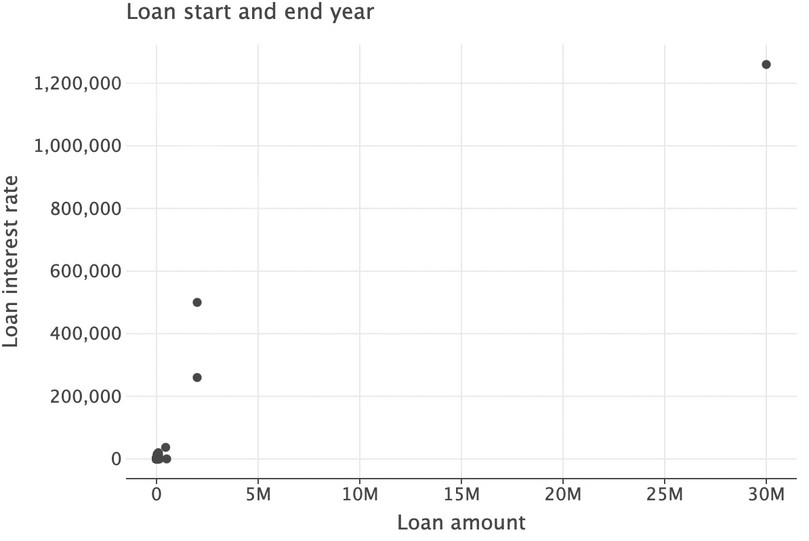
![]()
Figure 9.6 Scatterplot showing loan amounts and interest payments.
One large loan (top-right corner) dominates this graph. Let’s exclude observations with a loan amount larger than 200,000 from the plotted area of the graph.
(
    ggplot(got_l_c, aes(x="loan_amount", y="loan_interest"))
    + geom_point(size=3)
    + labs(
        title="Loan start and end year", x="Loan amount", y="Loan interest rate"
    )
    + ylim(0, 3e4)
    + xlim(0, 2e5)
)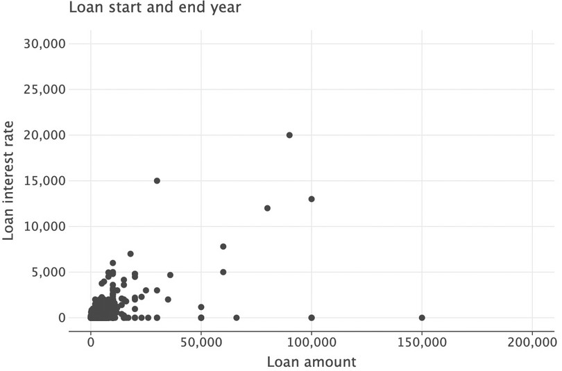
![]()
Figure 9.7 Revised scatterplot showing loan amounts and interest payments without outliers.
Interestingly, we can see many zero-interest loans. Now we will calculate the interest rate as
loan_interest/loan_amount.got_l_c["interest_rate"] = got_l_c["loan_interest"] / got_l_c["loan_amount"] got_l_c["interest_rate"].describe()count 1445.000000 mean 0.256616 std 5.262957 min 0.000000 25% 0.000000 50% 0.000000 75% 0.166667 max 200.000000 Name: interest_rate, dtype: float64The maximum interest rate is 200 (in other words, 20,000%), which does not make sense and could be due to a data entry error. Making another scatterplot can also identify extreme values for loan amounts:
(
    ggplot(got_l_c, aes(x="loan_amount", y="interest_rate"))
    + geom_point(size=3)
    + labs(
        title="Loan amounts and interest rates", x="Loan amount", y="Loan interest rate"
    )
)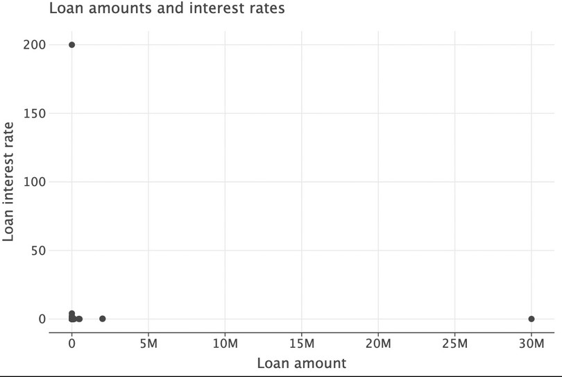
![]()
Figure 9.8 Scatterplot identifying extreme values for loan amounts.
Let’s make another scatterplot, excluding the observation with the extremely high interest rate and only looking at small loan amounts (less than 1,000).
(
    ggplot(got_l_c, aes(x="loan_amount", y="interest_rate"))
    + geom_point(size=3)
    + labs(
        title="Loan amounts and interest rates", x="Loan amount", y="Loan interest rate"
    )
    + xlim(0, 1e3)
    + ylim(0, 5)
)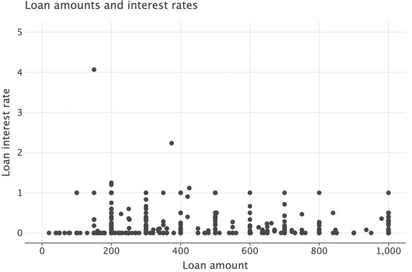
![]()
Figure 9.9 Scatterplot excluding extremely high interest rates and including only small loan amounts.
Again, we can see that there are many zero-interest loans. From the summary statistics above, we can see that the median interest rate is 0, which implies that at least 50% of loans have a zero interest rate. The following code calculates that percentage precisely.
num_zero_interest_rate = (
    100 * (got_l_c["interest_rate"] == 0).sum() / got_l_c["interest_rate"].count()
)

print(f"The number of loans with a rate of zero is {num_zero_interest_rate.round(2)}%")
The number of loans with a rate of zero is 50.52%Now let’s calculate statistics conditional on whether a loan is long term or not. Before we do this, we will remove the observation with the very extreme interest rate (20,000%) from our
got_l_cdataset (but not from the originalgot_ldataset). That observation has a loan amount of 1 and an interest payment of 200, which is probably a data entry mistake. There is another extreme observation (with a loan amount of 30,000,000), but there is no indication that this observation is misrecorded as there is a significant interest payment for this loan.got_l_c = got_l_c.loc[got_l_c["interest_rate"] < 200, :] got_l_c.groupby("long_term")["interest_rate"].agg( ["mean", "std", "min", "max", "median", "count"] ).round(2)
mean std min max median count long_term False 0.09 0.18 0.0 1.00 0.00 512 True 0.19 0.27 0.0 2.24 0.14 211 Both the mean and median interest rate are higher for long-term loans. You can adapt the code above to calculate statistics for the
loan_amountvariable.We now calculate correlations between interest rates and household characteristics. We store the correlation coefficients in a matrix (array of rows and columns) called
m_corr.m_corr = got_l_c.loc[ ~got_l_c["interest_rate"].isna(), [ "age", "max_education", "number_assets", "hhsize", "young_children", "working_age_adults", "interest_rate", ], ].corr() m_corr["interest_rate"].round(4)age 0.0258 max_education -0.0841 number_assets -0.0474 hhsize 0.1050 young_children 0.1022 working_age_adults 0.0466 interest_rate 1.0000 Name: interest_rate, dtype: float64
- Now we will look at sources of finance and how they are related to loan characteristics.
- Create a table showing the proportion of loans (in terms of the column variable) with source of finance (
borrowed_from) as the row variable andruralas the column variable. Make a similar table but withborrowed_from_otheras the row variable instead. Does it look like rural households use different sources of finance from urban households? (Hint: It may help to think about sources of finance in terms of formal, informal, and other institutions such as microfinancers or NGOs.)
-
For each of the variables below, create a table showing the average of that variable, with
borrowed_fromas the row variable andruralas the column variable. Comment on any similarities or differences between rows and columns that you find interesting, and suggest explanations for what you observe.- duration of loan (using the variable in which negative durations were transformed to positive durations)
- loan amount
- interest rate
- Create a table showing the proportion of
gender(in terms of the row variable) withborrowed_fromas the row variable andruralas the column variable. Describe any relationships you observe between the gender of household head, the place where he/she lives, and the types of finance used.
- What other variables are currently not in our dataset but could also be important for our analysis in Questions 2 and 3?
Python walk-through 9.11 Creating summary tables of means
First we use the
pd.crosstabmethod to create the table with the variableborrowed_from.stab_10 = pd.crosstab( got_l_c["borrowed_from"], got_l_c["rural"], margins=True, normalize="columns", ).round(4) stab_10
rural Large town (urban) Rural Small town (urban) All borrowed_from Bank (Commercial) 0.0188 0.0039 0.0000 0.0070 Employer 0.0408 0.0020 0.0103 0.0111 Grocery/Local Merchant 0.0815 0.0471 0.1031 0.0585 Microfinance Institution 0.1912 0.2797 0.2680 0.2592 Money Lender (Katapila) 0.0031 0.0481 0.0206 0.0362 NGO 0.0125 0.0471 0.0515 0.0397 Neighbour 0.1066 0.1158 0.0722 0.1108 Other (Specify) 0.0564 0.1207 0.0412 0.1010 Relative 0.4859 0.3150 0.4330 0.3610 Religious Institution 0.0031 0.0206 0.0000 0.0153 Note that in all settings, most loans come from relatives. To create the table with
borrowed_from_other, substitute this variable name in the above command.Let’s take a quick look at the loan lengths we expect (the mean) when looking at the cross-tab between
ruralandborrowed_from:tab_10 = got_l_c.groupby(["borrowed_from", "rural"])["loan_length_abs"].agg("mean") tab_10.head()borrowed_from rural Bank (commercial) Large town (urban) 1814 days 04:48:00 Rural 619 days 00:00:00 Small town (urban) NaT Employer Large town (urban) 602 days 00:00:00 Rural 289 days 12:00:00 Name: loan_length_abs, dtype: timedelta64[ns]We don’t need the extra information on hours in the last column, so let’s instead simplify the time information to only use full days. And we’ll ‘unstack’ the data to make it wider in format too, making it a bit more readable.
tab_10.dt.days.unstack()
rural Large town (urban) Rural Small town (urban) borrowed_from Bank (Commercial) 1,814.0 619.0 NaN Employer 602.0 289.0 NaN Grocery/Local Merchant 165.0 258.0 175.0 Microfinance Institution 712.0 410.0 509.0 Money Lender (Katapila) 365.0 331.0 365.0 NGO 372.0 395.0 236.0 Neighbour 124.0 186.0 296.0 Other (Specify) 273.0 371.0 806.0 Relative 237.0 216.0 392.0 Religious Institution 1,461.0 343.0 NaN
Extension: Investigating sources of finance associated with zero-interest loans
We previously saw that a large percentage of loans have a zero interest rate. Here we investigate whether particular sources of finance are responsible for these interest rates. The code we use is very similar to the code above, but instead of calculating the mean of a variable, we calculate the mean of a Boolean (true/false) variable (
interest_rate==0). This will deliver the proportion ofTrueobservations, in other words, loans where the interest rate was equal to zero.tab_11 = ( got_l_c.assign(rate_of_zero=lambda x: x["interest_rate"] == 0) .groupby(["borrowed_from", "rural"], dropna=False) .agg(prop_0_interest=("rate_of_zero", "mean")) .unstack() ) tab_11.round(2)
prop_0_interest rural Large town (urban) Rural Small town (urban) borrowed_from NaN 0.00 0.57 1.00 Bank (Commercial) 0.00 0.00 NaN Employer 0.69 0.50 1.00 Grocery/Local Merchant 1.00 0.81 1.00 Microfinance Institution 0.08 0.04 0.04 Money Lender (Katapila) 0.00 0.02 0.50 NGO 0.25 0.08 0.40 Neighbour 1.00 0.76 1.00 Other (Specify) 0.22 0.17 0.00 Relative 0.96 0.82 0.98 Religious Institution 1.00 0.19 NaN In both urban and rural settings, a high proportion of loans granted by local merchants, neighbours, and relatives are zero interest (possibly because these people have a close relationship with the borrower, so there is a lower chance of default).
We will use the same technique to determine the proportion of loans that go to households that report having a woman as the household head.
tab_12 = (
    got_l_c.assign(headed_by_woman=lambda x: x["gender"] == "Female")
    .groupby(["borrowed_from", "rural"], dropna=False)
    .agg(prop_women=("headed_by_woman", "mean"))
    .unstack()
)

tab_12.round(2)
prop_women rural Large town (urban) Rural Small town (urban) borrowed_from NaN 1.00 0.43 1.00 Bank (Commercial) 0.00 0.50 NaN Employer 0.31 0.00 0.00 Grocery/Local Merchant 0.38 0.19 0.50 Microfinance Institution 0.41 0.13 0.31 Money Lender (Katapila) 0.00 0.27 0.50 NGO 0.25 0.31 0.20 Neighbour 0.35 0.25 0.43 Other (Specify) 0.39 0.19 0.25 Relative 0.40 0.21 0.29 Religious Institution 1.00 0.24 NaN You can see that in both urban and rural settings, a high proportion of loans granted by local merchants, neighbours, and relatives are zero interest (possibly because these people have a close relationship with the borrower so there is a lower chance of default).
We will use exactly the same technique to determine the proportion of loans that go to households with female heads.
tab11 <- gotLc %>%
  group_by(borrowed_from, rural) %>%
  summarize(prop_female = mean((gender == "Female"),
    na.rm = TRUE)) %>%
  spread(rural, prop_female) %>%
  print()
## # A tibble: 11 x 4 ## # Groups: borrowed_from [11] ## borrowed_from `Large town (urban)` Rural `Small town (urban~ ## <fct> <dbl> <dbl> <dbl> ## 1 Bank (commercial) 0. 0.500 NA ## 2 Employer 0.308 0. 0. ## 3 Grocery/Local Merchant 0.385 0.188 0.500 ## 4 Microfinance Institution 0.410 0.130 0.308 ## 5 Money Lender (Katapila) 0. 0.265 0.500 ## 6 NGO 0.250 0.312 0.200 ## 7 Neighbour 0.353 0.254 0.429 ## 8 Other (specify) 0.389 0.187 0.250 ## 9 Relative 0.400 0.206 0.286 ## 10 Religious Institution 1.00 0.238 NA ## 11 <NA> 1.00 0.429 1.00
- In this project we have looked at patterns in borrowing and access to credit, but we are not able to make any causal statements such as ‘changes in X will cause households to be credit constrained’ or ‘characteristic Y causes improved access to credit’. Outline a policy intervention that could help improve households’ access to loans, and how to design the implementation so you can assess the causal effects of this policy.
