Extra Empirical Project 2: The politics of carbon taxation Solutions
These are not model answers. They are provided to help students, including those doing the project outside a formal class, to check their progress while working through the questions using the Excel, R, Google Sheets, or Python walk-throughs. There are also brief notes for the more interpretive questions. Students taking courses using Doing Economics should follow the guidance of their instructors.
Part 1: Measuring and explaining public support for carbon taxation
- All respondents in the survey (in other words, both the control and treatment groups) are provided with a short explanation of a carbon tax directly before they are asked about their level of support for the policy. The explanation goes through how a carbon tax operates, highlights that those who use more fossil fuel products will pay more, and links a carbon tax to tackling climate change. Informing respondents about carbon taxes is the step that the authors take to try to improve the accuracy of the information they receive from respondents on their level of support for the policy.
- There are 2,997 respondents in the dataset.
- There are 1,481 respondents in the treatment group. There are therefore 2,997 – 1,481 = 1,516 respondents in the control group.
- The authors recode the variable to be a dummy variable that takes the value of ‘1’ if respondents answered the carbon tax preferences question by saying that they ‘support’ or ‘strongly support’ a carbon tax, and is ‘0’ otherwise. An advantage of recoding the variable in this manner is that it is easier to interpret and is simplified for analysis (for example, in a regression model). The downside is that you lose some of the variation and detail in your carbon tax support variable (for example, you can no longer differentiate between respondents that ‘support’ and ‘strongly support’ a carbon tax). In other words, the dummy variable is not able to pick up the intensity of respondents’ support (or lack of support) for the policy.
- No solution needed.
Hint for those working in Excel: Creating the dummy variable for carbon tax support (while taking account of missing values) involves nesting an IF function within another IF function. The formula for the first data point for the carbon tax dummy variable should be:
=IF(G2="","",IF(OR(G2=1,G2=2),1,0). This formula can then be copied down to the other respondents in the dataset. The formula tells Excel to leave the cell blank if the respondent has not answered the question on carbon tax preferences (that is, if it is blank). If the respondent has answered the carbon tax preferences question, the formula then tells Excel to put a ‘1’ in the cell if the respondent has answered ‘1’ or ‘2’ for this question, indicating that they ‘strongly support’ or ‘support’ the policy, and to put ‘0’ in the cell if they have given any other answer.
- No solution needed.
Hint for those working in Excel: You can use similar formulas to the one outlined above to create the four dummy variables asked for in this question.
- No solution needed.
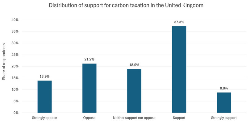
- Solution figure 1 shows how carbon tax support is distributed in the UK.
| Carbon tax support | Number of respondents | Percentage of respondents |
|---|---|---|
| Strongly oppose | 207 | 13.9% |
| Oppose | 317 | 21.2% |
| Neither support nor oppose | 282 | 18.9% |
| Support | 557 | 37.3% |
| Strongly support | 131 | 8.8% |
Solution figure 1 The distribution of carbon tax support in the UK.
- Solution figure 2 shows how carbon tax support is distributed in the UK (with data labels).
Solution figure 2 The distribution of carbon tax support in the UK.
- The modal (most common) answer to the question was ‘Support’, with 37.3% of respondents indicating this level of support for carbon taxation. Less than 10% of respondents (8.8%) indicated that they strongly supported the policy. Roughly a fifth (18.9%) were in the middle category, indicating a more neutral stance on carbon taxes. The remaining 35.1% of respondents indicated that they either opposed or strongly opposed carbon taxation. While this is less than the share of respondents showing support or strong support for the policy (46.1%), there is still a large chunk of the sample that is opposed to taxing carbon. This distribution of support highlights one of the key difficulties facing governments hoping to mitigate climate change through carbon taxation—it is unpopular with a sizeable share of the public.
- The average is 0.461 (or 46.1%). This is the same as the share of respondents that either ‘support’ or ‘strongly support’ carbon taxation in Solution figure 1.
- The average of the carbon tax dummy for a given subsample of the dataset can be interpreted as the share of respondents in that subsample that support or strongly support carbon taxation. In the case of Question 10(a), the average of this variable for the control group indicates that 46.1% of the control group are supportive of taxing carbon.
- Solution figure 3 is a table showing how average carbon tax support differs for respondents under 40, and those 40 and over.
| 0 = Aged under 40 | 1 = Aged 40 and over | |
|---|---|---|
| Average carbon tax support | 0.53 | 0.41 |
Solution figure 3 Average carbon tax support, by age group.
- Solution figure 4 is a table showing how average carbon tax support differs for respondents who commute by car and those who do not.
| 0 = Do not commute by car | 1 = Car commuters | |
|---|---|---|
| Average carbon tax support | 0.55 | 0.41 |
Solution figure 4 Average carbon tax support, by non-car commuters and car commuters.
- Solution figure 5 is a table showing how average carbon tax support differs for respondents living in rural areas and non-rural areas.
| 0 = Non-rural | 1 = Rural | |
|---|---|---|
| Average carbon tax support | 0.47 | 0.43 |
Solution figure 5 Average carbon tax support, by rurality.
- Solution figure 6 is a table showing how average carbon tax support differs for respondents who support different political parties.
| Average carbon tax support | |
|---|---|
| Conservative Party | 0.34 |
| Democratic Unionist Party | 0.75 |
| Green Party of England and Wales | 0.69 |
| Labour Party | 0.55 |
| Liberal Democrats | 0.53 |
| Other | 0.50 |
| Plaid Cymru | 0.33 |
| Prefer not to say | 0.26 |
| Reform UK | 0.17 |
| Scottish National Party | 0.62 |
| Sinn Féin | 0.38 |
Solution figure 6 Average carbon tax support, by political affiliation.
- The solution tables for Question 11 show that carbon tax support is on average higher for younger respondents, those who do not commute by car, and those living in non-rural areas. We also see that support varies dramatically by the political affiliation of the respondents. For example, support is low among respondents who feel closest to the Conservative Party (0.34) and Reform UK (0.17) and is high among respondents who feel closest to the Labour Party (0.55) and the Green Party (0.69).
While exposure to carbon taxes (for example, due to driving to work) appears to be associated with lower support, it is not just economic factors that are correlated with support levels. The largest difference in support across the tables in Question 11 is by respondents’ political affiliation. Overall, the tables highlight that there are demographic, economic, and political drivers of support for carbon taxes.
A wide range of other variables could be associated with respondents’ support for carbon taxes. Two possible examples are respondents’ scepticism about climate change (we would expect climate sceptics to be more opposed to carbon taxation) and respondents’ level of education (previous research has found that higher education levels tend to be associated with higher support for carbon taxation).
Part 2: Explaining rural backlashes against carbon taxation
- No solution needed.
- Solution figure 7 is a table showing how average carbon tax unfairness perceptions differ for rural respondents in the control group who perceive a high degree of unequal treatment (8 or above on the 0–10 scale) compared with those who do not.
| 0 = Low unequal treatment perceptions (7 and below) | 1 = High unequal treatment perceptions (8 and above) | |
|---|---|---|
| Average carbon tax unfairness perceptions | 5.1 | 6.2 |
Solution figure 7 Average carbon tax unfairness perceptions, by non-high and high unequal treatment perceptions.
- Solution figure 8 is a table showing how average carbon tax support differs for rural respondents in the control group who perceive a high degree of unequal treatment (8 or above on the 0–10 scale) compared with those who do not.
| 0 = Low unequal treatment perceptions (7 and below) | 1 = High unequal treatment perceptions (8 and above) | |
|---|---|---|
| Average carbon tax support | 0.47 | 0.41 |
Solution figure 8 Average carbon tax support, by non-high and high unequal treatment perceptions.
- Rural respondents who perceive a high degree of unequal treatment (by the UK government) tend to perceive carbon taxes as more unfair.
- They also express lower support for carbon taxation—47% of rural respondents with non-high unequal treatment perceptions support carbon taxation, whereas only 41% of rural respondents with high unequal treatment perceptions support carbon taxation.
- No solution needed.
- Solution figure 9 is a column chart showing how average unequal treatment perceptions differ for rural respondents in the control and treatment groups
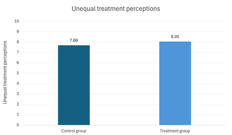
Solution figure 9 Average unequal treatment perceptions for rural respondents in the control and treatment groups.
- Solution figure 10 is a column chart showing how average carbon tax unfairness perceptions differ for rural respondents in the control and treatment groups
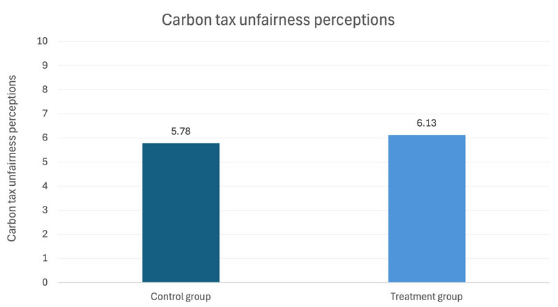
Solution figure 10 Average carbon unfairness perceptions for rural respondents in the control and treatment groups.
- Solution figure 11 is a column chart showing how average carbon tax support differs for rural respondents in the control and treatment groups.
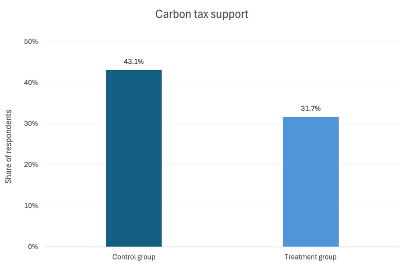
Solution figure 11 Average carbon tax support for rural respondents in the control and treatment groups.
- No solution needed.
- The p-value for the difference in means between the treatment and control groups for unequal treatment perceptions is 0.023.
- The p-value for the difference in means between the treatment and control groups for carbon tax fairness perceptions is 0.082.
- The p-value for the difference in means between the treatment and control groups for carbon tax support is 0.004.
- The p-values differ across the three variables. The lowest p-value is for carbon tax support and the highest p-value is for carbon tax fairness perceptions. For each of the three variables, the hypothesis being tested is that there is no difference in means between the treatment and control groups (in other words, that the information treatment did not affect the variable). The p-value tells us the probability of observing data at least as extreme as the data collected, if our hypothesis that there is no difference in means between the treatment and control groups is true. The smaller the p-value, the less likely that we would observe differences at least as extreme as those we did, given our hypothesis. Hence, the smaller the p-value, the lower the probability that the information treatment did not have an effect on the variable. For carbon tax support, the p-value is 0.004, which indicates that there is only a 0.4% probability of seeing differences at least as extreme as those observed in the experiment, given our hypothesis that there is no difference in means between the treatment and control groups. For this variable, the experiment therefore provides strong evidence that the information treatment reduced support for carbon taxation. The p-value for carbon tax fairness perceptions is 0.082 or 8.2%. While this is still statistically significant (at the 90% level), the evidence that there is a difference in means is weaker than it is for carbon tax support (or unequal treatment perceptions).
- Extension: The 95% confidence intervals for the difference in means for the three variables are:
- unequal treatment perceptions: [0.049, 0.667]
- carbon tax fairness perceptions: [–0.044, 0.732]
- carbon tax support: [–0.191, –0.037].
Solution figure 12 is a column chart showing the difference in means for rural respondents in the treatment and control groups for the three variables, including 95% confidence intervals.
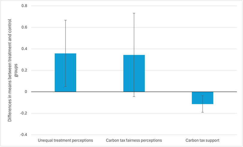
Solution figure 12 Differences in means (and confidence intervals) for rural respondents in the treatment and control groups.
The confidence intervals relate closely to the p-values calculated in Question 8. We can see that zero is included in the 95% confidence interval for carbon tax unfairness perceptions, which is aligned with the p-value being 0.082 (that is, only statistically significant at the 90% level). The confidence intervals for the other two variables do not include zero, so there is a smaller likelihood for these variables that there is no difference in means between the treatment and control groups (that is, that the information treatment did not affect the variables). The confidence interval for carbon tax support is the smallest, which also fits with it having the smallest p-value in Question 8.
There are many strengths and weaknesses of information provision experiments mentioned in the Haaland et al. (2023) article. Here are some examples:
Strengths:
- This is a powerful method to test economic theories and answer policy relevant questions.
- Randomizing respondents into treatment and control groups allows researchers to estimate causal effects of beliefs on outcomes.
- Information provision experiments can be fielded relatively easily and cheaply by researchers through online survey platforms or companies.
- There are applications across a wide range of different subfields in economics including public economics, political economy, macroeconomics, household finance, and labour, education, and health economics.
Weaknesses:
- Respondents could be inattentive and speed through online surveys, which lowers the quality of the answers received.
- Data quality could be affected by bots (automated computer programs) taking surveys on online survey platforms.
- Experimenter demand effects: Respondents could change their responses to the survey to align with what they believe the researcher expects or hypothesizes.
- Beliefs are difficult to measure accurately and there is no consensus on how best to elicit them in surveys (for example, through qualitative or quantitative survey questions).
- Here are some potential changes that could be made to the experiment in Hope et al. (2026):
- Alter the information provided to the treatment group (for example, an information treatment with data that directly shows urban–rural differences on per capita government spending in the UK).
- Increase the sample size: There are 613 rural respondents in the dataset. It would have increased the statistical power of the analysis to have a larger sample, especially for the observational analysis in the article, which only uses data from the control group.
- The measure of respondents’ rurality in the survey is subjective. In other words, respondents are asked to select whether they live in a rural, urban, or suburban area. An objective measure of rurality (for example, based on respondents’ location and definitions of rural areas from national statistical authorities) could have been used instead of or alongside the subjective measure.
- No solution needed. Answers will depend on the output of the generative-AI tool and answers to the previous parts of Question 10.
